

Active Optics System Simulations Using opSim and imSim#
This document outlines the steps needed to run opSim-sourced imSim simulations for the Rubin Observatory Active Optics System (AOS).
Last verified to run: 02/28/2024
Versions:
lsst_distrib w_2024_04 (ext, cvmfs)
ts_wep v8.3.0
ts_imsim v1.0.1
galsim 2.5.1
imsim v2.0 (commit e6124cfc from Jan 18th, 2024)
skycatalogs 1.7.0-rc2 (commit d0d0d58ae1e)
Setup on USDF#
We assume working at the USDF, with working installations of imSim (imSim, skyCatalogs) and AOS packages (ts_imsim, ts_wep). To work properly, imSim requires to use the cvmfs extended version of the LSST Science Pipelines. To run this notebook on the Rubin Science Platform
(RSP) with the AOS packages, we use a jupyter notebook with LSST kernel, adding the source /sdf/data/rubin/user/scichris/WORK/aos_packages/setup_aos.sh line in ${HOME}/notebooks/.user_setups
To use imsim and AOS packages at the USDF we setup:
>> source imsim-setup.sh
>> source aos-seup.sh
which contain:
imsim-setup.sh
#!/usr/bin/env bash
source /cvmfs/sw.lsst.eu/linux-x86_64/lsst_distrib/w_2024_02/loadLSST-ext.bash
setup lsst_distrib
export IMSIM_HOME=/sdf/data/rubin/user/scichris/WORK/imsim_home
export RUBIN_SIM_DATA_DIR=$IMSIM_HOME/rubin_sim_data
export SIMS_SED_LIBRARY_DIR=$IMSIM_HOME/rubin_sim_data/sims_sed_library
setup -k -r $IMSIM_HOME/imSim
setup -k -r $IMSIM_HOME/skyCatalogs
aos-setup.sh
#!/usr/bin/env bash
export PATH_TO_TS_WEP=/sdf/group/rubin/ncsa-home/home/scichris/aos/ts_wep/
export PATH_TO_TS_OFC=/sdf/group/rubin/ncsa-home/home/scichris/aos/ts_ofc/
export PATH_TO_TS_IMSIM=/sdf/data/rubin/user/scichris/WORK/aos_packages/ts_imsim/

eups declare -r $PATH_TO_TS_WEP -t $USER --nolocks
eups declare -r $PATH_TO_TS_OFC -t $USER --nolocks
eups declare -r $PATH_TO_TS_IMSIM -t $USER --nolocks

setup ts_ofc -t $USER  -t current
setup ts_wep -t $USER  -t current
setup ts_imsim -t $USER -t current

export LSST_ALLOW_IMPLICIT_THREADS=True
We import all needed packages:
[1]:
from lsst.ts.wep.utils import  runProgram
from lsst.ts.wep.utils import getConfigDir as getWepConfigDir
from lsst.ts.imsim.opd_metrology import OpdMetrology

import lsst.obs.lsst as obs_lsst
from lsst.afw.cameraGeom import FIELD_ANGLE
from lsst.meas.algorithms import ReferenceObjectLoader
import lsst.geom
from lsst.daf import butler as dafButler

from astropy.coordinates import angular_separation
from astropy.visualization import ZScaleInterval
from astropy.coordinates import SkyCoord
from astropy import units as u
from astropy.table import Table
from astropy.io import fits

import matplotlib.pyplot as plt
import matplotlib.patches as patches
import matplotlib.patheffects as pe

import numpy as np

import sqlite3
import numpy as np
import pandas as pd
from scipy.ndimage import rotate

pd.set_option('display.max_rows', 500)
pd.set_option('display.max_columns', 500)
Simulation setup#
Exploring opSim database#
We show how to inspect the opSim database that is used as a source of information about the telescope pointing (boresight), filter, scheduled time, and other observation parameters. We are using here baseline_v3.2_10yrs.
First we find visits scheduled between two specific dates. We show what is the time difference between successive visits, how they can be grouped, and how this grouping corresponds to a particular observing night.
[2]:
columns = '*' # select all columns

# query for all visits scheduled  between these dates
mjd_start = 61800
mjd_end = 62500

opsim_db_file = '/sdf/data/rubin/user/jchiang/imSim/rubin_sim_data/opsim_cadences/baseline_v3.2_10yrs.db'

query = (f"select {columns} from observations where "
         f" {mjd_start} < observationStartMJD "
         f"and observationStartMJD < {mjd_end} "
        )

with sqlite3.connect(opsim_db_file) as con:
    df0 = pd.read_sql(query, con)

tab = Table.from_pandas(df0)
print(len(tab))
384634
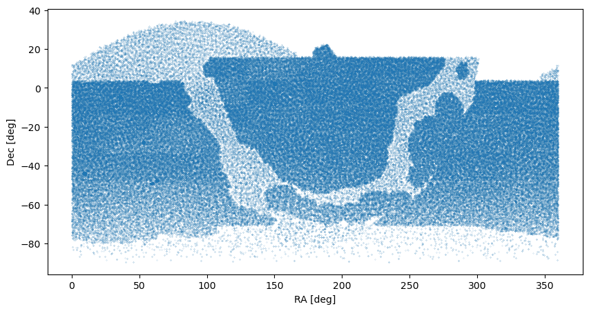
We plot the field pointings to illustrate that the visits span the region observable from the southern location of the observatory in Cerro Pachon. The region with less overall visits is the galactic plane.
[3]:
fig,ax = plt.subplots(figsize=(10, 5), dpi=100)
ax.scatter(tab['fieldRA'],tab['fieldDec'], s=0.01)
ax.set_xlabel('RA [deg]')
ax.set_ylabel('Dec [deg]')
[3]:
Text(0, 0.5, 'Dec [deg]')
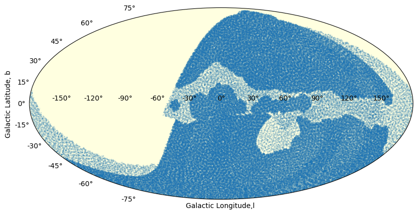
We illustrate that in galactic coordinates:
[4]:
fig = plt.figure(figsize=(10, 5), dpi=100)
ax = fig.add_subplot(111, projection='mollweide', facecolor ='LightYellow')
coords = SkyCoord(ra=tab['fieldRA'].value*u.degree,
                  dec=tab['fieldDec'].value*u.degree, frame='icrs')
longitude = coords.galactic.l.deg
latitude = coords.galactic.b.deg
# shift the scale : opSim 0, 360, and we want to go -180,180
ind = longitude > 180
longitude[ind] -=360    # scale conversion to [-180, 180]
longitude = - longitude   # reverse the scale: East to the left
ax.scatter(np.deg2rad(longitude), np.deg2rad(latitude),s=0.01)
ax.set_xlabel('Galactic Longitude,l ')
ax.set_ylabel('Galactic Latitude, b')
[4]:
Text(0, 0.5, 'Galactic Latitude, b')
[5]:
df0[:10]
[5]:
| observationId | fieldRA | fieldDec | observationStartMJD | flush_by_mjd | visitExposureTime | filter | rotSkyPos | rotSkyPos_desired | numExposures | airmass | seeingFwhm500 | seeingFwhmEff | seeingFwhmGeom | skyBrightness | night | slewTime | visitTime | slewDistance | fiveSigmaDepth | altitude | azimuth | paraAngle | cloud | moonAlt | sunAlt | note | target | fieldId | proposalId | block_id | observationStartLST | rotTelPos | rotTelPos_backup | moonAz | sunAz | sunRA | sunDec | moonRA | moonDec | moonDistance | solarElong | moonPhase | cummTelAz | scripted_id | |
|---|---|---|---|---|---|---|---|---|---|---|---|---|---|---|---|---|---|---|---|---|---|---|---|---|---|---|---|---|---|---|---|---|---|---|---|---|---|---|---|---|---|---|---|---|---|
| 0 | 620088 | 0.546178 | -35.466250 | 61800.029519 | 61800.052436 | 15.0 | i | 275.791864 | 0.0 | 1 | 1.786619 | 0.645924 | 1.159512 | 1.005119 | 18.215289 | 1004 | 112.417002 | 16.0 | 57.480105 | 22.007741 | 34.036195 | 245.374497 | 105.373386 | 0.0 | 6.407891 | -12.370712 | twilight_near_sun, 0 | -1 | 10 | 1 | 68.673633 | 21.16525 | 0.0 | 271.929209 | 240.612010 | 311.673930 | -17.941097 | 344.834636 | -1.714807 | 36.770580 | 46.497703 | 20.200751 | -114.625503 | 0 | |
| 1 | 620089 | 356.935778 | -36.270136 | 61800.029759 | 61800.052436 | 15.0 | i | 274.446672 | 0.0 | 1 | 1.939997 | 0.645924 | 1.218250 | 1.053402 | 18.071301 | 1004 | 4.719320 | 16.0 | 3.033959 | 21.868502 | 31.028528 | 243.357125 | 106.718578 | 0.0 | 6.334876 | -12.435441 | twilight_near_sun, 0 | -1 | 11 | 1 | 68.760200 | 21.16525 | 0.0 | 271.888075 | 240.560746 | 311.674177 | -17.941032 | 344.837051 | -1.713506 | 36.325400 | 43.769782 | 20.202140 | -116.502391 | 0 | |
| 2 | 620090 | 353.256188 | -36.995973 | 61800.029998 | 61800.052436 | 15.0 | i | 273.108964 | 0.0 | 1 | 2.105144 | 0.645924 | 1.279455 | 1.103712 | 17.950589 | 1004 | 4.723977 | 16.0 | 3.040449 | 21.739902 | 28.361106 | 241.520609 | 108.056286 | 0.0 | 6.261844 | -12.500149 | twilight_near_sun, 0 | -1 | 12 | 1 | 68.846786 | 21.16525 | 0.0 | 271.846933 | 240.509408 | 311.674424 | -17.940968 | 344.839467 | -1.712206 | 36.127880 | 41.085248 | 20.203530 | -118.315459 | 0 | |
| 3 | 620091 | 355.598991 | -39.190407 | 61800.030237 | 61800.052436 | 15.0 | i | 275.397987 | 0.0 | 1 | 1.958784 | 0.645924 | 1.225316 | 1.059209 | 18.106459 | 1004 | 4.657245 | 16.0 | 2.865973 | 21.877725 | 30.698519 | 239.701782 | 105.767263 | 0.0 | 6.189045 | -12.564614 | twilight_near_sun, 0 | -1 | 0 | 1 | 68.933094 | 21.16525 | 0.0 | 271.805924 | 240.458172 | 311.674670 | -17.940904 | 344.841878 | -1.710909 | 38.743323 | 43.469676 | 20.204916 | -120.109909 | 0 | |
| 4 | 620092 | 354.095265 | -42.077105 | 61800.030474 | 61800.052436 | 15.0 | i | 276.190494 | 0.0 | 1 | 1.982059 | 0.645924 | 1.234031 | 1.066373 | 18.058966 | 1004 | 4.430362 | 16.0 | 3.103925 | 21.844408 | 30.299882 | 236.100234 | 104.974756 | 0.0 | 6.117045 | -12.628336 | twilight_near_sun, 0 | -1 | 1 | 1 | 69.018454 | 21.16525 | 0.0 | 271.765366 | 240.407437 | 311.674914 | -17.940840 | 344.844263 | -1.709627 | 41.213784 | 43.304736 | 20.206288 | -123.690296 | 0 | |
| 5 | 620093 | 351.708899 | -39.880944 | 61800.030713 | 61800.052436 | 15.0 | i | 273.685844 | 0.0 | 1 | 2.137472 | 0.645924 | 1.291208 | 1.113373 | 17.976717 | 1004 | 4.636846 | 16.0 | 2.840305 | 21.739750 | 27.894327 | 237.916107 | 107.479406 | 0.0 | 6.044316 | -12.692668 | twilight_near_sun, 0 | -1 | 2 | 1 | 69.104676 | 21.16525 | 0.0 | 271.724398 | 240.356126 | 311.675160 | -17.940776 | 344.846675 | -1.708332 | 38.679175 | 40.843799 | 20.207674 | -121.855438 | 0 | |
| 6 | 620094 | 347.737179 | -40.452118 | 61800.030953 | 61800.052436 | 15.0 | i | 271.826670 | 0.0 | 1 | 2.354544 | 0.735720 | 1.500507 | 1.285417 | 17.823456 | 1004 | 4.756254 | 16.0 | 3.088071 | 21.480127 | 25.132350 | 236.216642 | 109.338580 | 0.0 | 5.971165 | -12.757338 | twilight_near_sun, 0 | -1 | 3 | 1 | 69.191397 | 21.16525 | 0.0 | 271.683194 | 240.304454 | 311.675407 | -17.940711 | 344.849102 | -1.707030 | 38.833446 | 38.271694 | 20.209069 | -123.532396 | 0 | |
| 7 | 620095 | 349.500444 | -37.624909 | 61800.031189 | 61800.052436 | 15.0 | i | 271.419123 | 0.0 | 1 | 2.330146 | 0.735720 | 1.491159 | 1.277732 | 17.748810 | 1004 | 4.404504 | 16.0 | 3.141279 | 21.452371 | 25.414114 | 239.644589 | 109.746128 | 0.0 | 5.899253 | -12.820877 | twilight_near_sun, 0 | -1 | 4 | 1 | 69.276649 | 21.16525 | 0.0 | 271.642689 | 240.253596 | 311.675650 | -17.940648 | 344.851489 | -1.705749 | 36.172771 | 38.441599 | 20.210442 | -120.080289 | 0 | |
| 8 | 620096 | 347.449214 | -35.319397 | 61800.031428 | 61800.052436 | 15.0 | i | 269.452918 | 0.0 | 1 | 2.560242 | 0.735720 | 1.577839 | 1.348983 | 17.791400 | 1004 | 4.642116 | 16.0 | 2.834630 | 21.389944 | 22.991094 | 241.341471 | 111.712332 | 0.0 | 5.826502 | -12.885122 | twilight_near_sun, 0 | -1 | 5 | 1 | 69.362893 | 21.16525 | 0.0 | 271.601712 | 240.202083 | 311.675896 | -17.940584 | 344.853906 | -1.704454 | 33.701424 | 36.109018 | 20.211831 | -118.358133 | 0 | |
| 9 | 620097 | 351.075974 | -34.739587 | 61800.031668 | 61800.052436 | 15.0 | i | 270.773027 | 0.0 | 1 | 2.323787 | 0.735720 | 1.488716 | 1.275724 | 17.953864 | 1004 | 4.711443 | 16.0 | 3.025676 | 21.556021 | 25.488633 | 243.076636 | 110.392223 | 0.0 | 5.753505 | -12.949547 | twilight_near_sun, 0 | -1 | 6 | 1 | 69.449427 | 21.16525 | 0.0 | 271.560599 | 240.150333 | 311.676143 | -17.940519 | 344.856333 | -1.703155 | 33.541140 | 38.771454 | 20.213225 | -116.594670 | 0 |
[6]:
df0.columns
[6]:
Index(['observationId', 'fieldRA', 'fieldDec', 'observationStartMJD',
       'flush_by_mjd', 'visitExposureTime', 'filter', 'rotSkyPos',
       'rotSkyPos_desired', 'numExposures', 'airmass', 'seeingFwhm500',
       'seeingFwhmEff', 'seeingFwhmGeom', 'skyBrightness', 'night', 'slewTime',
       'visitTime', 'slewDistance', 'fiveSigmaDepth', 'altitude', 'azimuth',
       'paraAngle', 'cloud', 'moonAlt', 'sunAlt', 'note', 'target', 'fieldId',
       'proposalId', 'block_id', 'observationStartLST', 'rotTelPos',
       'rotTelPos_backup', 'moonAz', 'sunAz', 'sunRA', 'sunDec', 'moonRA',
       'moonDec', 'moonDistance', 'solarElong', 'moonPhase', 'cummTelAz',
       'scripted_id'],
      dtype='object')
One of the more useful columns is night that contains a unique identifier of a given observing night.
We can confirm that all visits indeed correspond to the same night by calculating time difference between successive visits, and grouping visits that have dt less than a few hours (which would correspond to a daytime break):
[7]:
# calculate time difference
deltas = []
for i in range(len(df0)-1):
    deltas.append(df0['observationStartMJD'][i+1] - df0['observationStartMJD'][i])
deltas.append(0) # for the last entry
df0['dt'] = deltas


# create groups

groups = []
groupId = 0
for i in range(len(df0)):
    groups.append(groupId)
    if df0['dt'][i] > 0.1:  # dt in units of days, so 0.1 is  0.1*24 hrs = 2.4 hrs
        groupId += 1
df0['group'] = groups

# find how many visits in each group
groups, count = np.unique(df0['group'], return_counts=True)

count_dic = {}
for i in range(len(groups)):
    count_dic[groups[i]] = count[i]

# add a groupCount to the catalog
groupCount = []
for i in range(len(df0)):
    groupCount.append(count_dic[df0['group'][i]])
df0['groupCount'] = groupCount
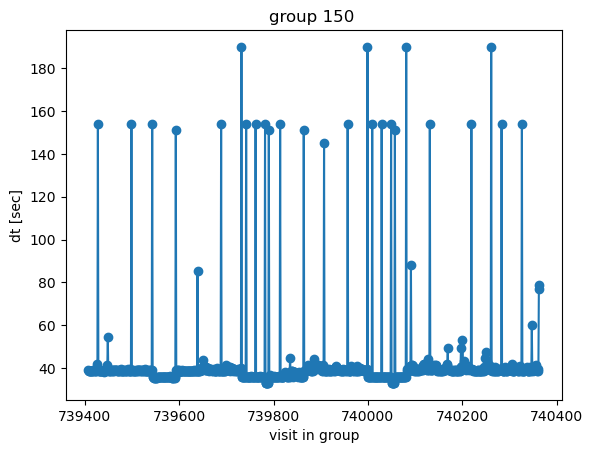
Select one group, and plot time difference between successive visits
[8]:
groupId=150
mask = (df0['group'] == groupId)# | (df0['group'] == groupId+1)
plt.plot(df0['observationId'][mask][:-1],  df0['dt'][mask][:-1]*24*3600,marker='o') # fraction of the day...
plt.ylabel('dt [sec]')
plt.xlabel('visit in group')
plt.title(f'group {groupId} ')
[8]:
Text(0.5, 1.0, 'group 150 ')
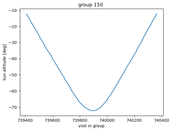
Also plot the behavior of sun altitude as the visits proceed:
[9]:
plt.title(f'group {groupId} ')
plt.plot(df0['observationId'][mask], df0['sunAlt'][mask])
plt.xlabel('visit in group')
plt.ylabel('Sun altitude [deg]')
[9]:
Text(0, 0.5, 'Sun altitude [deg]')
[10]:
np.unique(df0['night'][mask])
[10]:
array([1206])
This confirms that grouping visits by time difference corresponds to the same night. In this case, all grouped visits were from night 1206.
Choosing a visit#
Given the contents of the opSim database we can choose an appropriate visit / night given a variety of constraints. For example, to choose a visit close to a specific ra/dec location (which we set here as ra=20h 28min 18.74s and dec=-87deg 28min 19.9sec, like in DM-35005) we can do:
[11]:
# example sky coordinates
c0 = SkyCoord('20:28:18.74 -87:28:19.9', unit=(u.hourangle, u.deg))

# select all columns
columns = '*'

opsim_db_file = '/sdf/data/rubin/user/jchiang/imSim/rubin_sim_data/opsim_cadences/baseline_v3.2_10yrs.db'

ra0 = c0.ra.deg
dec0 =  c0.dec.deg
delta = 1 # deg  - maximum radial separation of catalog sources from selected position

query = (f"select {columns} from observations "
         f"where ({ra0 - delta} < fieldRA) "
         f"and (fieldRA < {ra0 + delta}) "
         f"and ({dec0 - delta} < fieldDec) "
         f"and (fieldDec < {dec0 + delta})")

with sqlite3.connect(opsim_db_file) as con:
    df0 = pd.read_sql(query, con)
[12]:
df0[['observationId','skyBrightness', 'moonDistance', 'moonPhase']]
[12]:
| observationId | skyBrightness | moonDistance | moonPhase | |
|---|---|---|---|---|
| 0 | 68609 | 22.577148 | 119.609695 | 20.754213 |
| 1 | 68659 | 22.030924 | 119.593130 | 20.551207 |
| 2 | 726966 | 18.626410 | 62.463349 | 72.526945 |
| 3 | 1429362 | 21.853259 | 70.949817 | 27.341871 |
| 4 | 1429412 | 20.789772 | 70.843448 | 27.115905 |
| 5 | 2032781 | 18.531647 | 109.194879 | 85.410819 |
| 6 | 2032831 | 19.033075 | 109.137269 | 85.291565 |
We see that even with such large allowance for pointing, only a few visits actually have a dark moon (phase < 30%) and good moon separation (>100 deg), so that lunar illumination doesn’t cause any additional background. The skyBrightness column reflects that: only 68659 and 68609 above have skyBrightness fainter than 22 mag.
Let’s choose 68659: ra=306.661504, dec=-86.924706 since it’s a particularly dark night (only 20% lunar phase, 120 deg away, and the sun is ~60 deg below the horizon.
[13]:
df0_select = df0[df0['observationId'].values == 68659]
[14]:
df0_select
[14]:
| observationId | fieldRA | fieldDec | observationStartMJD | flush_by_mjd | visitExposureTime | filter | rotSkyPos | rotSkyPos_desired | numExposures | airmass | seeingFwhm500 | seeingFwhmEff | seeingFwhmGeom | skyBrightness | night | slewTime | visitTime | slewDistance | fiveSigmaDepth | altitude | azimuth | paraAngle | cloud | moonAlt | sunAlt | note | target | fieldId | proposalId | block_id | observationStartLST | rotTelPos | rotTelPos_backup | moonAz | sunAz | sunRA | sunDec | moonRA | moonDec | moonDistance | solarElong | moonPhase | cummTelAz | scripted_id | |
|---|---|---|---|---|---|---|---|---|---|---|---|---|---|---|---|---|---|---|---|---|---|---|---|---|---|---|---|---|---|---|---|---|---|---|---|---|---|---|---|---|---|---|---|---|---|
| 1 | 68659 | 306.661504 | -86.924706 | 60907.246674 | 60907.251796 | 30.0 | g | 285.230776 | 285.230776 | 2 | 1.857446 | 0.589094 | 1.223033 | 1.057333 | 22.030924 | 111 | 9.405863 | 34.0 | 3.207455 | 24.179729 | 32.57299 | 182.354017 | 41.406847 | 0.0 | -43.117107 | -66.027409 | pair_33, ug, b | -1 | 81 | 1 | 346.8805 | -33.362377 | -47.621862 | 80.618694 | 134.791048 | 149.333306 | 12.46765 | 112.861448 | 26.609109 | 119.59313 | 105.302361 | 20.551207 | -48.434874 | 0 |
[15]:
ra_select =  df0_select['fieldRA'].values[0]
dec_select =  df0_select['fieldDec'].values[0]
night_select = df0_select['night'].values[0]
Find another visit that’s from the same night, within 10 degrees, also in g-filter :
[16]:
delta = 10 # degrees

query = (f"select {columns} from observations "
         f"where ({ra_select - delta} > fieldRA) "
         f"and (fieldRA < {ra_select + delta}) "
         f"and ({dec_select - delta} < fieldDec) "
         f"and (fieldDec < {dec_select + delta})"
        f"and filter=='g'"
        f"and night=={night_select}")
with sqlite3.connect(opsim_db_file) as con:
    df1 = pd.read_sql(query, con)
Find out how close these visits are:
[17]:
sep_deg=[]
for i in range(len(df1)):
    sep = angular_separation(ra_select*u.deg,dec_select*u.deg, df1['fieldRA'][i]*u.deg, df1['fieldDec'][i]*u.deg)
    sep_deg.append(np.rad2deg(sep))
df1['sep_deg'] = sep_deg
df1 = df1.sort_values('sep_deg')
[18]:
df1[['observationId', 'sep_deg', 'fieldRA', 'fieldDec','filter']]
[18]:
| observationId | sep_deg | fieldRA | fieldDec | filter | |
|---|---|---|---|---|---|
| 0 | 68661 | 5.675480077892328 deg | 293.785092 | -81.367774 | g |
| 1 | 68664 | 8.507424880771477 deg | 291.976271 | -78.553061 | g |
Ok, in this case we may want to choose visit 68661 as our second field since it is closer to the original visit.
Creating the imSim yaml config file#
Given the instrument and visit number we can simulate the visit sourced from the opSim catalog using a single yaml config file. Then the single call galsim imsim_config.yaml would run the simulation. An example imsim_config.yaml file that uses opSim database as an input is:
modules: [imsim]
template: imsim-config-skycat

# Use skyCatalogs for obtaining the objects to render.
input.sky_catalog:
  file_name: /sdf/home/s/scichris/link_to_scichris/WORK/imsim_home/skyCatalogs_v2/skyCatalog.yaml
  #file_name: /sdf/data/rubin/user/jchiang/imSim/skyCatalogs_v2/skyCatalog.yaml
  approx_nobjects: 1500
  band: { type: OpsimData, field: band }
  mjd: { type: OpsimData, field: mjd }
  obj_types: [gaia_star]
  max_flux: 1e9

input.opsim_data.file_name: /sdf/data/rubin/user/jchiang/imSim/rubin_sim_data/opsim_cadences/baseline_v3.2_10yrs.db
input.opsim_data.visit: 740000

input.atm_psf.screen_size: 819.2
input.atm_psf.save_file:
  type: FormattedStr
  format: atm_psf_files/atm_psf_%08d-%1d-%s.pkl
  items:
      - { type: OpsimData, field: observationId }
      - { type: OpsimData, field: snap }
      - { type: OpsimData, field: band }

# offset the piston by 1.5 mm
input.telescope.focusZ: 0   # telescope offset is in meters

# disable checkpointing
input.checkpoint: ""

image.random_seed: '@input.opsim_data.visit'

# enlarge the stamp size
#  to avoid cutting off donut edges
image.stamp_size: 300
stamp.size: 300

# disable FFT
stamp.fft_sb_thresh: 0


# simulate no objects for OPD-only
#image.nobjects: 0

output.nproc: 120
output.nfiles: 205
output.det_num: {type: Sequence, nitems: 205}

# make no amp images
#output.readout: ""

output.header:
    focusZ: 0.0   # header is in mm
    seqnum: 941

output.camera: LsstCam
output.dir:
    type: FormattedStr
    format : output/%08d
    items:
        - "@input.opsim_data.visit"

# create OPD at all LsstFAM CCD center  locations
# sorted by detId

output.opd:
    file_name:
        type: FormattedStr
        format: opd_%s.fits.fz
        items:
            - "@input.telescope.focusZ"
    rotTelPos:  "@input.telescope.rotTelPos"
    fields:
    - thx: -0.9403333333333335 deg
      thy: -1.6458888888888887 deg
    - thx: -0.7056111111111111 deg
      thy: -1.6458888888888887 deg
    - thx: -0.470888888888889 deg
      thy: -1.645888888888889 deg
    - thx: -0.9403333333333336 deg

    # apply specific formatting to the amp images
output.readout.file_name:
    type: FormattedStr
    format : amp_%08d-%1d-%s-%s-det%03d-%s.fits.fz
    items:
        - "@input.opsim_data.visit"  # eg. 00740000
        - 0   # snap
        - $band  # eg. g
        - $det_name  # eg. R22_S10
        - "@output.det_num"  # eg. 91--> 091
        - "@input.telescope.focusZ" #  eg. 0.0015

output.timeout: 1e5
output.truth.dir: '@output.dir'
output.truth.file_name.format: centroid_%08d-%1d-%s-%s-det%03d.txt.gz
Elements of this imsim_config.yaml file would be specific to what instrument is used. Below we comment on individual elements of this yaml file. Any of this settings can be overridden during the galsim call, with eg. galsim imsim_config.yaml input.opsim_data.visit=76543.
-> imported modules:
modules: [imsim]
template: imsim-config-skycat
are imported modules and templates. The location of imsim-config-skycat depends on the installation location of imsim, i.e. $imsim-home, for instance $imsim_home/imSim/config/imsim-config-skycat.yaml.
–> input.sky_catalog: input.sky_catalog: is the source of object catalog; it instructs imSim to obtain input source catalog by querying opSim.
The input.sky_catalog.file_name is the location of the yaml config file for querying the opSim database. An important component of that config is where to find the GAIA reference catalogs to obtain the source catalog. One way is to point to the main shared butler repository - the repo/main. In /sdf/data/rubin/user/jchiang/imSim/skyCatalogs_v2/skyCatalog.yaml
gaia_star:
    area_partition: None
    butler_parameters:
      collections: HSC/defaults
      dstype: gaia_dr2_20200414
      repo: /repo/main
    data_file_type: butler_refcat
    sed_method: use_lut
However, it suffers from a bottleneck where only a limited number of connections to a butler repo are allowed at any given time. If simulating hundreds of visits at the same time, other users may be querying /repo/main at the same time, and when limit is reached an error psycopg2.OperationalError: SSL connection has been closed unexpectedly will close connection and interrupt the simulation.
One way to avoid that /repo/main bottleneck of a number of allowed connections is to ingest the GAIA refcat to a standalone location (see this notebook for an example of GAIA refcat ingestion). An example skyCatalog.yaml could point either to a user-generated repo that contains GAIA refcat (eg. /sdf/group/rubin/shared/scichris/DM-41019/gen3repo), or to an AOS-shared
repo with GAIA refcat (eg. /sdf/group/rubin/repo/aos_imsim). For example, we could have:
gaia_star:
area_partition: None
butler_parameters:
  collections: refcats/gaia_dr2_20200414
  dstype: gaia_dr2_20200414
  repo: /sdf/group/rubin/repo/aos_imsim
data_file_type: butler_refcat
sed_method: use_lut
–> input.sky_catalog.approx_nobjects is an approximation provided to galsim to do preparation in setting up multiprocessing, and is used to speed up staging of the individual CCD processes.( J. Chiang, priv.comm.)
–> input.sky_catalog.obj_types: [gaia_star] limits the type of simulated objects to stars only (eg. excluding galaxies).
–> input.sky_catalog.max_flux sets the maximum allowed flux of a simulated source, it is a bright-end magnitude cutoff. “The flux units are e- , converted from photons by the CCD QE - this is essentially the total number of photons detected by the CCD from a given object”(J.Chiang, priv.comm.). The value max_flux:1e10 is about 10.5 magnitude cutoff, and 1e7 removes all sources brighter than ~13th mag.
–> input.opsim_data.visit is the opSim visit number. Like all parameters, it can be overridden during the galsim call
–> input.atm_psf.save_file pertains to the naming pattern of the atmospheric PSF files. These are 3.1 GB per visit, so one needs to ensure sufficient disk space. They can be easily re-created (do not need to be stored).
–> input.telescope.focusZ : the offset applied to the detector in meters, so 1.5 mm translates to 0.0015 m
–> image.stamp_size: 300, stamp.size: 300 - given that the donut postage stamp image is 160x160 px for LsstCam defocal offset of 1.5mm, this ensures that the stamp size for simulating a single source is larger than that. Otherwise we risk running into donuts that have square edges (as they did not fit in the default stamp).
–> stamp.fft_sb_thresh: 0 : this is needed to ensure that the FFT mode is turned off. Otherwise sources above that flux limit would be treated with the faster FFT, but that assumes that they are in-focus, which would produce in-focus brighter stars together with defocal fainter donuts. In the template: imsim-config-skycat config, it is set to 2e5, which is why we need to override it.
–> output.nproc: 120: the number of processes allocated to galsim; it is able to use only 1 processor per CCD, so unfortunately setting output.nproc to be larger than output.nfiles (number of output files) will not help. I.e. simulating only 9 CCDs output.nfiles: 9 with output.nproc: 18 would mean that while 9 processors are used, 9 are idle. Galsim is not able to split 1 CCD per multiple processors. The upper limit for output.nproc is the amount of available cores. On
USDF, many milano or ampere nodes have only 120 cores, so output.nproc: 120 corresponds to the upper limit. This means that if simulating output.nfiles:205, 120 will be simulated at the same time on 120 cores, and once these are finished, the next batch of 85 remaining CCDs will get simulated. Another strategy would be to minimize the number of idle cores, by setting the nproc so that the remnant of integer division of nfiles by nproc is as close to zero as
possible (eg. with nfiles:205, setting nproc:103 ensures that as few cores are idle as possible).
–> output.det_num this specifies which detectors should be simulated . For example, * output.det_num: {type: Sequence, nitems: 205} with output.nfiles:205 and output.camera: LsstCam simulates all LSSTCam Full Array Mode science sensors and corner wavefront sensors * output.det_num.first: 0 with output.nfiles: 9 and output.camera: LsstComCam simulates all 9 rafts on the LSSTComCam * output.det_num: {type: Sequence, nitems: 9} with output.nfiles: 9 and
output.camera: LsstComCam simulates all 9 rafts on the LSSTComCam * output.det_num: [191, 192, 195, 196, 199, 200, 203, 204] with output.nfiles: 8 and output.camera: LsstCam simulates only the corner wavefront sensors on LSSTCam
–> output.header specifies elements of the FITS header for the output amplifier files. For each visit, we want to store the focusZ (in mm) and seqNum. This is because the butler ingests images given their observation timestamp (dayObs) , and the sequence number seqNum , so that simulations based on the identical visit number but different focusZ need to be distinguished by their seqNum. The exposure number is constructed as eg. 5028081800960, with
50 corresponding to simulated imsim images (controller), 280818 simulated date (here 18th of August 2028), and 00960 the sequence number.
One possibility is to set seqNum to be N for the largest defocal offset in the negative direction, and increase N by 1 for each step in the focusing sequence, eg. focusZ:-1.5 is seqNum:940, then focusZ:0 is seqNum:941, and focusZ:1.5 is seqNum:942. This can be extended for more fine-grained focus sequences, eg.
focusZ: [-1.5,-1.25,-1.0,-0.75,-0.5,-0.25, 0, 0.25, 0.5, 0.75, 1.0, 1.25,1.5]
seqNum: [1, 2, 3, 4, 5, 6, 7, 8, 9, 10, 11, 12, 13]   or

seqNum: [941, 942, 943, 945, 946...]
one only needs to ensure that there aren’t two identical seqNums in the same observing day. The maximum seqNum is 99999 because it is assumed that the camera will not take more than 100,000 images in a single night (with 43,200 seconds in a 12hr night this corresponds to maximum of 0.5 exposures per second, which is 30 times greater than the planned cadence (of 2x15sec exposures back-to-back per filter, i.e. 1 exposure every 15 seconds). The typical opSim cadence produces about
1000-1500 images per night.
Therefore it is worth noting that using opSim cadence and assumed focus ‘sweep’ by eg. LSSTComCam (3 focusZ positions, [-1.5, 0, 1.5] mm) per opSim visit will produce three times more seqNums than usual, eg. given 1000 visits (pointings) per night, we simulate 3000 exposures (3 exposures per visit, each with different focusZ).
–> output.camera: LsstCam specifies the instrument to use (LsstCam or LsstComCam)
–> output.opd.fields specifies the field position (in degrees) of where to evaluate the optical path difference (OPD). This needs to be provided per instrument, and can be eg. centers of each CCD, or only 31 Gaussian quadrature points, or the mid-point of corner wavefront sensors… An example code is included in the section below.
–> output.readout.file_name specifies the file naming pattern for the written amplifier image. In this example we include the value of focusZ in each image name so that images sourced on the same visit do not get overwritten:
format : amp_%08d-%1d-%s-%s-det%03d-%s.fits.fz
    items:
        - "@input.opsim_data.visit"  # eg. 00740000
        - 0   # snap
        - $band  # eg. g
        - $det_name  # eg. R22_S10
        - "@output.det_num"  # eg. 91--> 091
        - "@input.telescope.focusZ" #  eg. 0.0015
translates to eg. amp_00068659-0-g-R22_S00-det090-0.0015.fits.fz
–> output.timeout: 1e5 specifies the value of galsim timeout in seconds. The default value of 3600 sec (1 hr per CCD) is insufficient in some cases.
–> output.truth.file_name.format: centroid_%08d-%1d-%s-%s-det%03d.txt.gz specifies the name of the centroid file that contains positions of all sources per image. Since the same sources are used per focusZ position it is not necessary to store separate focusZ per image. These files are useful to get eg. source count per image independent of the ISR and source detection or querying the reference catalog
Defining OPD field locations#
Here we provide short code snippets that provide various desirable field locations to evaluate OPD
LSSTComCam : center of each of the nine rafts
[19]:
camera =  obs_lsst.LsstComCam().getCamera()
detectors = list(camera.getNameMap().keys())

xps, yps = [],[]
for name in detectors:
    detector = camera.get(name)
    xp_rad, yp_rad = detector.getCenter(FIELD_ANGLE)  # in radians
    xp_deg, yp_deg =  np.rad2deg(xp_rad), np.rad2deg(yp_rad)

    print(name, detector.getId(), xp_deg, yp_deg)
    xps.append(xp_deg)
    yps.append(yp_deg)

# print in a format expected by imsim
i=0
print("\n")
for name in detectors:
    print("    - thx:", xps[i], "deg")
    print("      thy:", yps[i], "deg ")#"# ", name)
    i+=1
R22_S21 7 -5.555555555556424e-05 0.2346666666666667
R22_S20 6 -0.23477777777777778 0.2346666666666667
R22_S12 5 0.23466666666666663 -5.55555555555445e-05
R22_S11 4 -5.555555555556424e-05 -5.55555555555445e-05
R22_S10 3 -0.23477777777777778 -5.55555555555445e-05
R22_S22 8 0.23466666666666663 0.2346666666666667
R22_S02 2 0.23466666666666663 -0.23477777777777772
R22_S01 1 -5.555555555556424e-05 -0.2347777777777777
R22_S00 0 -0.23477777777777784 -0.23477777777777772


    - thx: -5.555555555556424e-05 deg
      thy: 0.2346666666666667 deg
    - thx: -0.23477777777777778 deg
      thy: 0.2346666666666667 deg
    - thx: 0.23466666666666663 deg
      thy: -5.55555555555445e-05 deg
    - thx: -5.555555555556424e-05 deg
      thy: -5.55555555555445e-05 deg
    - thx: -0.23477777777777778 deg
      thy: -5.55555555555445e-05 deg
    - thx: 0.23466666666666663 deg
      thy: 0.2346666666666667 deg
    - thx: 0.23466666666666663 deg
      thy: -0.23477777777777772 deg
    - thx: -5.555555555556424e-05 deg
      thy: -0.2347777777777777 deg
    - thx: -0.23477777777777784 deg
      thy: -0.23477777777777772 deg
LSSTCam: center of each 189 CCDs. In the snippet below we only plot the first few detectors:
[20]:
camera =  obs_lsst.LsstCam().getCamera()
all_detectors = list(camera.getNameMap().keys())

xps, yps = [],[]
detIds = []
for name in all_detectors:
    detector = camera.get(name)
    detId = detector.getId()
    # xp, yp = detector.getCenter(FOCAL_PLANE) # in mm
    xp_rad, yp_rad = detector.getCenter(FIELD_ANGLE)  # in radians
    xp_deg =  np.rad2deg(xp_rad)
    yp_deg = np.rad2deg(yp_rad)

    xps.append(xp_deg)
    yps.append(yp_deg)
    detIds.append(detId)

dets = Table([all_detectors, detIds, xps, yps], names=['detName', 'detId', 'xps', 'yps'])
dets.sort('detId')

print(dets[:4])

# print in a format expected by imsim
i=0
for row in dets[:4]:
    print("    - thx:", row['xps'], "deg")
    print("      thy:", row['yps'], "deg ")#"# ", name)
    i+=1
detName detId         xps                 yps
------- ----- ------------------- -------------------
R01_S00     0 -0.9403333333333335 -1.6458888888888887
R01_S01     1 -0.7056111111111111 -1.6458888888888887
R01_S02     2  -0.470888888888889  -1.645888888888889
R01_S10     3 -0.9403333333333336 -1.4111666666666667
    - thx: -0.9403333333333335 deg
      thy: -1.6458888888888887 deg
    - thx: -0.7056111111111111 deg
      thy: -1.6458888888888887 deg
    - thx: -0.470888888888889 deg
      thy: -1.645888888888889 deg
    - thx: -0.9403333333333336 deg
      thy: -1.4111666666666667 deg
LSSTCam: mid-point of the corner wavefront sensors
[21]:
camera =  obs_lsst.LsstCam().getCamera()

all_detectors = list(camera.getNameMap().keys())
wfs_detectors = [name for name in all_detectors if 'SW' in name]

xps, yps = [],[]
detIds = []
for name in wfs_detectors:
    detector = camera.get(name)
    detId = detector.getId()
    xp_rad, yp_rad = detector.getCenter(FIELD_ANGLE)  # in radians
    xp_deg =  np.rad2deg(xp_rad)
    yp_deg = np.rad2deg(yp_rad)
    #print(name, detector.getId(), xp_deg, yp_deg)
    xps.append(xp_deg)
    yps.append(yp_deg)
    detIds.append(detId)


dets = Table([wfs_detectors, detIds, xps, yps], names=['detName', 'detId', 'xps', 'yps'])
dets.sort('detId')

# Since we sorted the table with `detId` we only need to calculate the mid-point using two consecutive rows:
i = 0
xps_mids = []
yps_mids = []
while i < len(dets)-1:
    xi, xii = dets['xps'][i],  dets['xps'][i+1]
    yi, yii = dets['yps'][i],  dets['yps'][i+1]
    xps_mid = np.mean([xi,xii])
    yps_mid = np.mean([yi, yii])
    print(dets['detName'][i], dets['detName'][i+1], 'mid-point')
    print(xps_mid, yps_mid)
    xps_mids.append(xps_mid)
    yps_mids.append(yps_mid)
    i = i+2
    print('\n')

# print in a format expected by imsim
i=0
print("\n")
for i in range(len(xps_mids)):
    print("    - thx:", xps_mids[i], "deg")
    print("      thy:", yps_mids[i], "deg ") #"# ", name)
    i+=1
R00_SW0 R00_SW1 mid-point
-1.1902777777777778 -1.1902777777777778


R04_SW0 R04_SW1 mid-point
1.1902777777777778 -1.1902777777777778


R40_SW0 R40_SW1 mid-point
-1.1902777777777778 1.1902777777777778


R44_SW0 R44_SW1 mid-point
1.1902777777777778 1.1902777777777778


    - thx: -1.1902777777777778 deg
      thy: -1.1902777777777778 deg
    - thx: 1.1902777777777778 deg
      thy: -1.1902777777777778 deg
    - thx: -1.1902777777777778 deg
      thy: 1.1902777777777778 deg
    - thx: 1.1902777777777778 deg
      thy: 1.1902777777777778 deg
Running a simulation with slurm#
The imsim_config.yaml can be run as a single batch submission, eg.
srun --mem=28GB --cpus-per-task=4 galsim imsim_config.yaml
Or as an sbatch submission with the runSlurm.sl batch file. Following https://developer.lsst.io/usdf/batch.html the slurm file can be eg.
#!/bin/bash -l
#SBATCH --partition milano
#SBATCH --account rubin:developers
#SBATCH --nodes 1
#SBATCH --mem=100G
#SBATCH --cpus-per-task=9
#SBATCH -t 100:00:00
#SBATCH --job-name 950
#SBATCH --output=/sdf/data/rubin/shared/scichris/DM-41679_lsstComCam/slurm_68659_950.out
echo "starting at `date` on `hostname`"
pwd
galsim /sdf/data/rubin/shared/scichris/DM-41679_lsstComCam/imsim-run-R22-defocal_stamp_noFFT.yaml input.opsim_data.visit=68659        input.telescope.focusZ=-0.0015 output.header.focusZ=-1.5  output.header.seqnum=950

echo "ended at `date` on `hostname`"
The code snippet below generates such submission scripts for two visits, with three defocal offsets each.
[22]:
nodes=1
thrs = 100 # hrs for some jobs 5 hrs this is insufficient
partition='milano'
mem = 100 # GB, should be generally output.nproc*6GB , so here 9*6GB = 54 GB
cpus_per_task = 9


def write_to_file(out_file, content):
    with open(out_file, "w") as output:
        for line in content:
            output.write(line)
# Note that in the output directory we need to make the `atm_psf_files`
# directory (it doesn't get made automatically, as eg `output_all_R22` with the amp files does):
path_cwd = '/sdf/data/rubin/shared/scichris/DM-41679_lsstComCam/'
atm_files_dir = os.path.join(path_cwd, 'atm_psf_files')
if not os.path.exists(atm_files_dir):
    os.makedirs(atm_files_dir)

path_to_imsim_yaml = os.path.join(path_cwd, 'imsim-run-R22-defocal_stamp_noFFT.yaml')


visits = [68661,68659 ]
seqNumStart = [940, 950]

for visit, seqNum in zip(visits, seqNumStart):
    offsets_mm = 1e-3* np.array([-1.5, 0, 1.5]) # offsets in mm
    for focusz_mm in  offsets_mm :

        print(visit, seqNum,  focusz_mm)

        slurm_file = os.path.join(path_cwd, f'runSlurm-{visit}-{seqNum}.sl')

        # the instance catalog to use ...

        cmd = f"galsim {path_to_imsim_yaml} input.opsim_data.visit={visit}\
        input.telescope.focusZ={focusz_mm} output.header.focusZ={1000*focusz_mm}\
        output.header.seqnum={seqNum}"

        path_to_slurm_log = os.path.join(path_cwd, f'slurm_{visit}_{seqNum}.out')
        content = ['#!/bin/bash -l \n',
                  f'#SBATCH --partition {partition} \n',
                  '#SBATCH --account rubin:developers \n',
                  f'#SBATCH --nodes {nodes} \n',
                  f'#SBATCH --mem={mem}G \n',
                  f'#SBATCH --cpus-per-task={cpus_per_task}\n',
                  f'#SBATCH -t {thrs}:00:00 \n',
                  f'#SBATCH --job-name {seqNum} \n'
                  f'#SBATCH --output={path_to_slurm_log} \n',
                    'echo "starting at `date` on `hostname`" \n',
                    "pwd \n",
                     cmd,
                    '\n echo "ended at `date` on `hostname`" \n',
                  ]
        write_to_file(slurm_file, content)
        print(slurm_file)
        seqNum += 1 # ensure it's different for each defocal offset
68661 940 -0.0015
/sdf/data/rubin/shared/scichris/DM-41679_lsstComCam/runSlurm-68661-940.sl
68661 941 0.0
/sdf/data/rubin/shared/scichris/DM-41679_lsstComCam/runSlurm-68661-941.sl
68661 942 0.0015
/sdf/data/rubin/shared/scichris/DM-41679_lsstComCam/runSlurm-68661-942.sl
68659 950 -0.0015
/sdf/data/rubin/shared/scichris/DM-41679_lsstComCam/runSlurm-68659-950.sl
68659 951 0.0
/sdf/data/rubin/shared/scichris/DM-41679_lsstComCam/runSlurm-68659-951.sl
68659 952 0.0015
/sdf/data/rubin/shared/scichris/DM-41679_lsstComCam/runSlurm-68659-952.sl
These files can be submitted to slurm via
sbatch runSlurm-68661-940.sl
If more slurm files need to be submitted than 50-100, a script that staggers submissions to avoid overloading butler with refcat queries may be employed:
import subprocess
import os
import time

fpattern = 'runSlurm-'
flist = [f  for f in os.listdir(os.getcwd()) if f.startswith(fpattern) ]

batch_size = 25

Ntot = len(flist) # length of flist, so index runs from 0 to len(flist)-1


sleep_time_sec = 5*60 # 5 mins ...
c = 0 # batch count to start from ...
stop = 0 # initial value of stop (in case we start from the beginning)
while stop < Ntot:
    start = c*batch_size
    stop = (c+1)*batch_size
    print(start, stop)
    # catch the edge case where we've got only few visits left to run through ...
    if stop > Ntot:
        stop = Ntot
    for i in range(start,stop):
        slurm_file = flist[i]
        print(f"Running sbatch   {slurm_file}")
        subprocess.call(["sbatch", slurm_file])
    # wait after this batch has been submitted before submitting the next one ...
    print(f'Waiting {sleep_time_sec/60.} mins')
    time.sleep(sleep_time_sec)
    c+=1
Note - that code would need to be submitted from the USDF submission node. If it is stored in submit_staggered.py, it could be run with
python submit_staggered.py
Data analysis#
Creating a butler repository with GAIA refcats#
The following code snippet creates a gen3 butler repository and ingests GAIA reference catalog. These steps have already been performed for the shared AOS repo /sdf/group/rubin/repo/aos_imsim, but are repeated here to illustrate how refcats can be ingested to a standalone repository.
[23]:
path_cwd = '/sdf/data/rubin/shared/scichris/DM-41679_lsstComCam/'
butlerRootPath = os.path.join(path_cwd, f'gen3repo')

cmd = f"butler create {butlerRootPath}"
print(cmd)

cmd =f"butler register-instrument {butlerRootPath} lsst.obs.lsst.LsstComCam"
print(cmd)

ecsvPath = "/sdf/group/rubin/datasets/refcats/htm/v1/gaia_dr2_20200414.ecsv"
collection = "refcats/gaia_dr2_20200414"
datasetType = "gaia_dr2_20200414"

cmd = f"butler register-dataset-type {butlerRootPath} {datasetType} SimpleCatalog htm7"
print('\n',cmd)

cmd = f"butler ingest-files -t direct {butlerRootPath} {datasetType} {collection}  {ecsvPath} --prefix /sdf/group/rubin"
print(cmd)

cmd = f"butler collection-chain {butlerRootPath} --mode extend refcats {collection}"
print(cmd)
butler create /sdf/data/rubin/shared/scichris/DM-41679_lsstComCam/gen3repo
butler register-instrument /sdf/data/rubin/shared/scichris/DM-41679_lsstComCam/gen3repo lsst.obs.lsst.LsstComCam

 butler register-dataset-type /sdf/data/rubin/shared/scichris/DM-41679_lsstComCam/gen3repo gaia_dr2_20200414 SimpleCatalog htm7
butler ingest-files -t direct /sdf/data/rubin/shared/scichris/DM-41679_lsstComCam/gen3repo gaia_dr2_20200414 refcats/gaia_dr2_20200414  /sdf/group/rubin/datasets/refcats/htm/v1/gaia_dr2_20200414.ecsv --prefix /sdf/group/rubin
butler collection-chain /sdf/data/rubin/shared/scichris/DM-41679_lsstComCam/gen3repo --mode extend refcats refcats/gaia_dr2_20200414
Ingesting calibrations#
To analyse simulated raw images we need to write calibration files. These will be used to perform automatic reduction of the raw data as part of the instrument signature removal (ISR) process.
[24]:
butlerRootPath = os.path.join(path_cwd, f'gen3repo')
cmd = f"butler write-curated-calibrations {butlerRootPath} lsst.obs.lsst.LsstComCam"
print(cmd)
butler write-curated-calibrations /sdf/data/rubin/shared/scichris/DM-41679_lsstComCam/gen3repo lsst.obs.lsst.LsstComCam
Ingesting raw images#
After running the simulation we need to ingest the raw images to butler
[25]:
visits = [68661,68659 ]
path_cwd = '/sdf/data/rubin/shared/scichris/DM-41679_lsstComCam/'
butlerRootPath = os.path.join(path_cwd, f'gen3repo')
butlerInstName = "ComCam"
for visit in visits:
    outputImgDir = os.path.join(path_cwd, f'output', f'000{visit}')
    cmd=f"butler ingest-raws {butlerRootPath} {outputImgDir}/amp*"
    print('\n',cmd)


cmd = f"butler define-visits {butlerRootPath} lsst.obs.lsst.Lsst{butlerInstName}"
print('\n', cmd)
 butler ingest-raws /sdf/data/rubin/shared/scichris/DM-41679_lsstComCam/gen3repo /sdf/data/rubin/shared/scichris/DM-41679_lsstComCam/output/00068661/amp*

 butler ingest-raws /sdf/data/rubin/shared/scichris/DM-41679_lsstComCam/gen3repo /sdf/data/rubin/shared/scichris/DM-41679_lsstComCam/output/00068659/amp*

 butler define-visits /sdf/data/rubin/shared/scichris/DM-41679_lsstComCam/gen3repo lsst.obs.lsst.LsstComCam
Running ISR#
Given that we simulate both defocal and in-focus images, we run ISR on all images, and then run WEP only on pairs of defocal images.
[26]:
def writeWepConfigurationIsrOnly(instName, pipelineYamlPath, butlerInstName):
        """Write wavefront estimation pipeline task configuration.

        Parameters
        ----------
        instName : str
            Name of the instrument this configuration is intended for
            (lsst, lsstfam, comcam).
        pipelineYamlPath : str
            Path where the pipeline task configuration yaml file
            should be saved.
        butlerInstName : str
            Cam or ComCam, used to create appropriate `lsst.obs.lsst{butlerInstName}`
            instrument name, eg. `Cam` creates `lsstCam`.
        """

        with open(pipelineYamlPath, "w") as fp:
            fp.write(
                f"""# This yaml file is used to define the tasks and configuration of
# a Gen 3 pipeline used for testing
description: ISR-only pipeline
# Specify the corresponding instrument
instrument: lsst.obs.lsst.Lsst{butlerInstName}
# Specify each task in our pipeline by a name
# and then specify the class name corresponding to that task
tasks:
  isr:
    class: lsst.ip.isr.isrTask.IsrTask
    # Below we specify the configuration settings we want to use
    # when running the task in this pipeline. Since our data doesn't
    # include bias or flats we only want to use doApplyGains and
    # doOverscan in our isr task.
    config:
      connections.outputExposure: 'postISRCCD'
      doBias: False
      doVariance: False
      doLinearize: False
      doCrosstalk: False
      doDefect: False
      doNanMasking: False
      doInterpolate: False
      doBrighterFatter: False
      doDark: False
      doFlat: False
      doApplyGains: True
      doFringe: False
      doOverscan: True
      python: OverscanCorrectionTask.ConfigClass.fitType = 'MEDIAN'
"""
            )
instName = 'comcam'
pipelineYamlPath = os.path.join(path_cwd, "lsstPipelineISR.yaml")
butlerInstName = 'ComCam'
writeWepConfigurationIsrOnly(instName, pipelineYamlPath, butlerInstName)
print('Saved ', pipelineYamlPath)
Saved /sdf/data/rubin/shared/scichris/DM-41679_lsstComCam/lsstPipelineISR.yaml
Here we construct the pipetask call. With the working example we have two visits, three seqNums each, i.e. six exposures, all on the same opSim night. Thus we can capture all raws with exposure.day_obs dataset qualifier.
[27]:
isrRunName = 'runIsr'
numPro=5
pipelineYamlPath = os.path.join(path_cwd, "lsstPipelineISR.yaml")
day_obs = 20250820

print('\n')
bname = f'gen3repo'
butlerRootPath = os.path.join(path_cwd, bname)
cmd = f"pipetask run -b {butlerRootPath} "\
      f"-i LSST{butlerInstName}/raw/all,LSST{butlerInstName}/calib/unbounded "\
      f"--instrument lsst.obs.lsst.Lsst{butlerInstName} "\
      f"--register-dataset-types --output-run {isrRunName}  -p {pipelineYamlPath} -d "\
      f'"exposure.day_obs={day_obs}" -j {numPro}'

print(cmd)
pipetask run -b /sdf/data/rubin/shared/scichris/DM-41679_lsstComCam/gen3repo -i LSSTComCam/raw/all,LSSTComCam/calib/unbounded --instrument lsst.obs.lsst.LsstComCam --register-dataset-types --output-run runIsr -p /sdf/data/rubin/shared/scichris/DM-41679_lsstComCam/lsstPipelineISR.yaml -d "exposure.day_obs=20250820" -j 5
Running WEP as a pipetask#
We create pipeline configuration files to run the Wavefront Estimation Pipeline (WEP), with defocal sources (donuts) selected either using a process based on the reference catalog (via generateDonutCatalogWcsTask), or direct source detection (generateDonutDirectDetectTask).
[28]:
def writeWepConfigurationWcs(instName, pipelineYamlPath, butlerInstName):
        """Write wavefront estimation pipeline task configuration.

        Parameters
        ----------
        instName : str
            Name of the instrument this configuration is intended for
            (lsst, lsstfam, comcam, or auxtel).
        pipelineYamlPath : str
            Path where the pipeline task configuration yaml file
            should be saved.
        butlerInstName : str
            Cam or ComCam, used to create appropriate `lsst.obs.lsst{butlerInstName}`
            instrument name, eg. `Cam` creates `lsstCam`,
            `ComCam` creates `lsstComCam`
        """


        with open(pipelineYamlPath, "w") as fp:
            fp.write(
                f"""# This yaml file is used to define the tasks and configuration of
# a Gen 3 pipeline used for testing
description: WCS-based refcat donut selection and Zk estimation
# Here we specify the corresponding instrument for the data we
# will be using.
instrument: lsst.obs.lsst.Lsst{butlerInstName}
# Specify each task in our pipeline by a name
# and then specify the class name corresponding to that task
tasks:
  generateDonutCatalogWcsTask:
    class: lsst.ts.wep.task.generateDonutCatalogWcsTask.GenerateDonutCatalogWcsTask
    config:
    # this config points to the GAIA DR2 refcat
      connections.refCatalogs: gaia_dr2_20200414
      anyFilterMapsToThis: phot_g_mean
      donutSelector.useCustomMagLimit: True
      donutSelector.magMax: 15.0
      donutSelector.magMin: 11.0
      donutSelector.unblendedSeparation: 160
  cutOutDonutsScienceSensorTask:
    class: lsst.ts.wep.task.cutOutDonutsScienceSensorTask.CutOutDonutsScienceSensorTask
    config:
      # Obscuration (inner_radius / outer_radius of M1M3)
      instObscuration: 0.61
      # Focal length in m
      instFocalLength: 10.312
      # Aperture diameter in m
      instApertureDiameter: 8.36
      # Defocal distance offset in mm
      instDefocalOffset: 1.5
      # Camera pixel size in m
      instPixelSize: 10.0e-6
  calcZernikesTask:
    class: lsst.ts.wep.task.calcZernikesTask.CalcZernikesTask
    config:
      # Obscuration (inner_radius / outer_radius of M1M3)
      instObscuration: 0.61
      # Focal length in m
      instFocalLength: 10.312
      # Aperture diameter in m
      instApertureDiameter: 8.36
      # Defocal distance offset in mm
      instDefocalOffset: 1.5
      # Camera pixel size in m
      instPixelSize: 10.0e-6
    """)


pipelineYamlPath = os.path.join(path_cwd, "lsstPipelineWEPwcs.yaml")
writeWepConfigurationWcs(instName, pipelineYamlPath, 'ComCam')
print('Saved ', pipelineYamlPath)
Saved /sdf/data/rubin/shared/scichris/DM-41679_lsstComCam/lsstPipelineWEPwcs.yaml
We also run the direct detection of donuts; the magnitude limits are inspired by the WEP requirements.
[29]:
def writeWepConfigurationDirectDetect(instName, pipelineYamlPath, butlerInstName):
        """Write wavefront estimation pipeline task configuration.

        Parameters
        ----------
        instName : str
            Name of the instrument this configuration is intended for
            (lsst, lsstfam, comcam, or auxtel).
        pipelineYamlPath : str
            Path where the pipeline task configuration yaml file
            should be saved.
        butlerInstName : str
            Cam or ComCam, used to create appropriate `lsst.obs.lsst{butlerInstName}`
            instrument name, eg. `Cam` creates `lsstCam`,
            `ComCam` creates `lsstComCam`
        """


        with open(pipelineYamlPath, "w") as fp:
            fp.write(
                f"""# This yaml file is used to define the tasks and configuration of
# a Gen 3 pipeline used for testing
description: donut direct detection and Zk estimation
# Here we specify the corresponding instrument for the data we
# will be using.
instrument: lsst.obs.lsst.Lsst{butlerInstName}
# Specify each task in our pipeline by a name
# and the class name corresponding to that task
tasks:
  generateDonutDirectDetectTask:
    class: lsst.ts.wep.task.generateDonutDirectDetectTask.GenerateDonutDirectDetectTask
    config:
      instObscuration: 0.61
      instFocalLength: 10.312
      instApertureDiameter: 8.36
      instDefocalOffset: 1.5
      # instDefocalOffset: 0 for corner sensors
      instPixelSize: 10.0e-6
      donutSelector.useCustomMagLimit: True
      donutSelector.magMax: 16.0
  cutOutDonutsScienceSensorTask:
    class: lsst.ts.wep.task.cutOutDonutsScienceSensorTask.CutOutDonutsScienceSensorTask
    config:
      # Obscuration (inner_radius / outer_radius of M1M3)
      instObscuration: 0.61
      # Focal length in m
      instFocalLength: 10.312
      # Aperture diameter in m
      instApertureDiameter: 8.36
      # Defocal distance offset in mm
      instDefocalOffset: 1.5
      # Camera pixel size in m
      instPixelSize: 10.0e-6
  calcZernikesTask:
    class: lsst.ts.wep.task.calcZernikesTask.CalcZernikesTask
    config:
      # Obscuration (inner_radius / outer_radius of M1M3)
      instObscuration: 0.61
      # Focal length in m
      instFocalLength: 10.312
      # Aperture diameter in m
      instApertureDiameter: 8.36
      # Defocal distance offset in mm
      instDefocalOffset: 1.5
      # Camera pixel size in m
      instPixelSize: 10.0e-6
    """)


pipelineYamlPath = os.path.join(path_cwd, "lsstPipelineWEPdirect.yaml")
writeWepConfigurationDirectDetect(instName, pipelineYamlPath, 'ComCam')
print('Saved ', pipelineYamlPath)
Saved /sdf/data/rubin/shared/scichris/DM-41679_lsstComCam/lsstPipelineWEPdirect.yaml
Note that we defined explicitly the instrument-specific settings, but in the AOS pipeline they are imported via:
imports:
    - location: {getWepConfigDir()}/cwfs/instData/{instName}/instParamPipeConfig.yaml
In the two visits simulated here we chose 940 and 950 as starting seqNum. We thus have two pipetask calls to run WEP on each pair of defocal images:
[30]:
inputRun = isrRunName

for wep in ['wcs','direct']:
    pipelineYamlPath = os.path.join(path_cwd, f"lsstPipelineWEP{wep}.yaml")
    for seqNumStart in [940,950]:
        seqNumIntra = seqNumStart
        seqNumExtra = seqNumStart+2
        outputRun = f'runWEP_{seqNumIntra}-{seqNumExtra}_{wep}'

        cmd = f"pipetask run -b {butlerRootPath} "+\
                    f"-i refcats/gaia_dr2_20200414,{inputRun},LSST{butlerInstName}/calib/unbounded "+\
                f"--instrument lsst.obs.lsst.Lsst{butlerInstName} "+\
                f"--register-dataset-types --output-run {outputRun}  -p {pipelineYamlPath} -d "+\
            f'"exposure.seq_num in ({seqNumIntra},{seqNumExtra}) " -j {numPro}'
        print('\n',cmd)
 pipetask run -b /sdf/data/rubin/shared/scichris/DM-41679_lsstComCam/gen3repo -i refcats/gaia_dr2_20200414,runIsr,LSSTComCam/calib/unbounded --instrument lsst.obs.lsst.LsstComCam --register-dataset-types --output-run runWEP_940-942_wcs  -p /sdf/data/rubin/shared/scichris/DM-41679_lsstComCam/lsstPipelineWEPwcs.yaml -d "exposure.seq_num in (940,942) " -j 5

 pipetask run -b /sdf/data/rubin/shared/scichris/DM-41679_lsstComCam/gen3repo -i refcats/gaia_dr2_20200414,runIsr,LSSTComCam/calib/unbounded --instrument lsst.obs.lsst.LsstComCam --register-dataset-types --output-run runWEP_950-952_wcs  -p /sdf/data/rubin/shared/scichris/DM-41679_lsstComCam/lsstPipelineWEPwcs.yaml -d "exposure.seq_num in (950,952) " -j 5

 pipetask run -b /sdf/data/rubin/shared/scichris/DM-41679_lsstComCam/gen3repo -i refcats/gaia_dr2_20200414,runIsr,LSSTComCam/calib/unbounded --instrument lsst.obs.lsst.LsstComCam --register-dataset-types --output-run runWEP_940-942_direct  -p /sdf/data/rubin/shared/scichris/DM-41679_lsstComCam/lsstPipelineWEPdirect.yaml -d "exposure.seq_num in (940,942) " -j 5

 pipetask run -b /sdf/data/rubin/shared/scichris/DM-41679_lsstComCam/gen3repo -i refcats/gaia_dr2_20200414,runIsr,LSSTComCam/calib/unbounded --instrument lsst.obs.lsst.LsstComCam --register-dataset-types --output-run runWEP_950-952_direct  -p /sdf/data/rubin/shared/scichris/DM-41679_lsstComCam/lsstPipelineWEPdirect.yaml -d "exposure.seq_num in (950,952) " -j 5
If we wanted to only test WEP on a subset of detectors we could add eg. detector in (2,3) to the data query.
If we simulated all science and wavefront sensors but wanted to run WEP only on science sensors we can select these with detector.purpose = 'SCIENCE'. Likewise, we can choose only the wavefront sensors with detector.purpose = 'WAVEFRONT'.
Rerun with donutSelector.unblendedSeparation: 160
pipetask run -b /sdf/data/rubin/shared/scichris/DM-41679_lsstComCam/gen3repo -i refcats/gaia_dr2_20200414,runIsr,LSSTComCam/calib/unbounded --instrument lsst.obs.lsst.LsstComCam --register-dataset-types --output-run runWEP_940-942_direct_ -p /sdf/data/rubin/shared/scichris/DM-41679_lsstComCam/lsstPipelineWEPdirect.yaml -d "exposure.seq_num in (940,942) " -j 5
To allow more interaction with the intermediate data products it is also possible to run WEP tasks in the notebook. The following notebooks explain the steps needed to run the tasks, from source (donut) selection, creating donut cutouts (postage stamp images), to Zernike mode wavefront estimation: - source selection with WCS - source selection using direct detection - source selection using pointing information - creating donut cutouts - wavefront estimation
Running WEP with bps#
For multiple visits and detectors, running with bps (batch processing system) ensures that the butler to which we are storing the outputs does not get overwhelmed with the number of direct SQL queries.
Following BPS documentation we first create at USDF a file ~/.lsst/condor-info.py, containing (instead of $USERNAME enter the USDF username below):
config.platform["s3df"].user.name="$USERNAME"
config.platform["s3df"].user.home="/sdf/home/s/$USERNAME"
Then we run allocateNodes.py,
allocateNodes.py -v -n 10 -c 64 -m 60:00:00 -q roma,milano -g 1800 s3df --account rubin:commissioning
That allocates 10 nodes with 64 CPUs each for 60 hrs. If no jobs are submitted within 1800sec the glide-in allocation expires and alocateNodes.py has to be re-run.
Following the guide we create /sdf/group/rubin/shared/scichris/DM-41679_lsstComCam/site_bps.yaml containing
site:
  s3df:
    profile:
      condor:
        +Walltime: 7200
The pipetask
pipetask run -b {path_to_butler} -i {input_collections} --instrument lsst.obs.lsst.LsstComCam --register-dataset-types --output-run {run_name} -p {path_to_yaml} -d {data_query} -j 10
where input_collections includes {refcat_collection}{isr_collection}{calibration_collection}
translates to
bps submit site_bps.yaml -b {path_to_butler} -i {input_collections} -o {run_name} -p {path_to_yaml} -d {data_query} --extra-init-options "--instrument lsst.obs.lsst.LsstCam --register-dataset-types"
For example,
bps submit site_bps.yaml -b /sdf/data/rubin/shared/scichris/DM-41679_lsstComCam/gen3repo -i refcats/gaia_dr2_20200414,runIsr,LSSTComCam/calib/unbounded -o runWEP_950-952_bps -p /sdf/data/rubin/shared/scichris/41679_lsstComCam/lsstPipelineWEP.yaml -d "exposure.seq_num in (950,952)"
Reading centroid files#
The centroid files can be useful to for instance count the number of objects that are included in the image
[31]:
path_cwd = '/sdf/group/rubin/shared/scichris/DM-41679_lsstComCam'
fpath = os.path.join(path_cwd,'output-max-flux-1e9', '00068661', 'centroid_00068661-0-g-R22_S00-det000.txt.gz')
centroid = Table.read(fpath, format='csv',delimiter=' ',
          names=['object_id','ra','dec','x','y','nominal_flux','phot_flux','fft_flux','realized_flux'])
print(centroid[:10])
print('\n Total number of objects in this CCD is ', len(centroid))
         object_id               ra         dec     ... fft_flux realized_flux
---------------------------- ---------- ----------- ... -------- -------------
gaia_dr2_6359790450097863808 295.745998  -81.713754 ...      0.0       11052.0
gaia_dr2_6359790587536812544 295.476082 -81.7115474 ...      0.0       58138.0
gaia_dr2_6359790591832646656 295.537112 -81.7145562 ...      0.0        7184.0
gaia_dr2_6359790621896552448 295.597561 -81.7135217 ...      0.0       15514.0
gaia_dr2_6359790626193117056 295.606109 -81.7091303 ...      0.0      975303.0
gaia_dr2_6359790656256301056  295.74687 -81.6964621 ...      0.0       43371.0
gaia_dr2_6359790660552852096 295.675964 -81.6996442 ...      0.0       35622.0
gaia_dr2_6359790690616183168 295.578422  -81.708226 ...      0.0       16380.0
gaia_dr2_6359790694912595200 295.585394  -81.706379 ...      0.0     1262015.0
gaia_dr2_6359790694912595968 295.571472 -81.6972657 ...      0.0    40122023.0

 Total number of objects in this CCD is  683
[32]:
mean_centroid_ra = np.mean(centroid['ra'])
mean_centroid_dec = np.mean(centroid['dec'])
print(f"mean ra={mean_centroid_ra}, dec={mean_centroid_dec}" )
mean ra=295.39614332357246, dec=-81.59774462532943
Plotting reference catalog source locations#
We can query the reference catalog to obtain the source locations used by galsim to simulate the visit. Note that the fieldRA, fieldDec present in the FITS header correspond to the pointing of the visit (boresight), i.e. the center of the field of view. This means that these correspond exactly to the center of R22_S11 since that’s the central raft, but for the corner sensors, it is better to use the centroid file corresponding to a given corner sensor, and calculate the mean of the
ra , dec of objects in that sensor. This is what we do in this example:
[33]:
mean_ra_deg = mean_centroid_ra
mean_dec_deg = mean_centroid_dec


collection='refcats/gaia_dr2_20200414'
dstype='gaia_dr2_20200414'
butlerRootPath = os.path.join(path_cwd, 'gen3repo')
butler = dafButler.Butler(butlerRootPath,
                           collections=['refcats/gaia_dr2_20200414'])
refs = set(butler.registry.queryDatasets(dstype))

refCats = [dafButler.DeferredDatasetHandle(butler, _, {})
           for _ in refs]


dataIds = [butler.registry.expandDataId(_.dataId) for _ in refs]
config = ReferenceObjectLoader.ConfigClass()
config.filterMap = {f'{_}': f'phot_{_}_mean' for _ in ('g', 'bp', 'rp')}
ref_obj_loader = ReferenceObjectLoader(dataIds=dataIds,
                                       refCats=refCats,
                                       config=config)

ra = lsst.geom.Angle(mean_ra_deg, lsst.geom.degrees)
dec = lsst.geom.Angle(mean_dec_deg, lsst.geom.degrees)

center = lsst.geom.SpherePoint(ra, dec)
radius = lsst.geom.Angle(1500, lsst.geom.arcseconds)
refcat_region = lsst.sphgeom.Circle(center.getVector(), radius)
band = 'bp'
cat = ref_obj_loader.loadRegion(refcat_region, band).refCat
df = cat.asAstropy().to_pandas().sort_values('id')
INFO:lsst.meas.algorithms.loadReferenceObjects.ReferenceObjectLoader:Loading reference objects from None in region bounded by [292.54347830, 298.24880834], [-82.01441301, -81.18107624] RA Dec
INFO:lsst.meas.algorithms.loadReferenceObjects.ReferenceObjectLoader:Loaded 7278 reference objects
[34]:
df[:4]
[34]:
| id | coord_ra | coord_dec | phot_g_mean_flux | g_camFlux | phot_bp_mean_flux | bp_camFlux | phot_rp_mean_flux | rp_camFlux | phot_g_mean_fluxErr | g_camFluxErr | phot_bp_mean_fluxErr | bp_camFluxErr | phot_rp_mean_fluxErr | rp_camFluxErr | coord_raErr | coord_decErr | epoch | pm_ra | pm_dec | pm_raErr | pm_decErr | pm_flag | parallax | parallaxErr | parallax_flag | astrometric_excess_noise | phot_variable_flag | |
|---|---|---|---|---|---|---|---|---|---|---|---|---|---|---|---|---|---|---|---|---|---|---|---|---|---|---|---|---|
| 2227 | 6347682559333342336 | 5.141738 | -1.431137 | 60349.333720 | 60349.333720 | 48042.776329 | 48042.776329 | 91550.212451 | 91550.212451 | 183.098984 | 183.098984 | 2187.133629 | 2187.133629 | 2374.512800 | 2374.512800 | 1.287502e-09 | 1.468586e-09 | 57205.874409 | 1.076734e-09 | -3.436459e-08 | 2.591071e-09 | 2.905852e-09 | False | 1.230859e-09 | 1.568164e-09 | False | 0.00000 | NOT_AVAILABLE |
| 2002 | 6347682559333401472 | 5.142896 | -1.431161 | 51250.534104 | 51250.534104 | 32040.119818 | 32040.119818 | 104398.748146 | 104398.748146 | 177.869842 | 177.869842 | 2092.624943 | 2092.624943 | 2335.022543 | 2335.022543 | 1.465456e-09 | 1.686865e-09 | 57205.874409 | 2.479213e-08 | -7.536406e-08 | 3.005054e-09 | 3.323866e-09 | False | 6.124334e-10 | 1.740461e-09 | False | 0.00000 | NOT_AVAILABLE |
| 2091 | 6347682563630378240 | 5.142940 | -1.431073 | 120788.564772 | 120788.564772 | 62069.016586 | 62069.016586 | 222106.934921 | 222106.934921 | 235.845794 | 235.845794 | 2068.664712 | 2068.664712 | 2481.203986 | 2481.203986 | 8.612467e-10 | 9.634437e-10 | 57205.874409 | -3.792447e-09 | 4.519851e-08 | 1.790965e-09 | 1.841551e-09 | False | 2.784224e-09 | 1.039702e-09 | False | 0.47975 | NOT_AVAILABLE |
| 2092 | 6347682563630378368 | 5.142853 | -1.431118 | 490539.308596 | 490539.308596 | 251022.902296 | 251022.902296 | 887274.733654 | 887274.733654 | 344.012632 | 344.012632 | 2648.685341 | 2648.685341 | 4366.685086 | 4366.685086 | 2.990641e-10 | 3.473743e-10 | 57205.874409 | 2.056232e-08 | 4.182208e-08 | 6.042890e-10 | 6.245315e-10 | False | 5.148430e-09 | 3.821001e-10 | False | 0.08107 | NOT_AVAILABLE |
Find out which elements of the refcat are also cointained in the centroid file for that particular detector:
[35]:
centroid_ids = [int(object_id.split('_')[2]) for object_id in centroid['object_id']]
centroid['ids'] = centroid_ids

# this confirms that all centroid  sources are in obtained refcat
# since the source catalog originated from the refcat,
# a sufficiently large query radius will provide a subset of the refcat
# that encompasses all the centroid sources
# if this was not true, we may need to query for a slightly larger region
# than 1500 sec above to obtain all refcat sources
assert np.sum(np.in1d(centroid['ids'] , df['id'] )) == len(centroid)

# this creates a boolean mask to tell us which of the refcat sources got simulated
df['simulated'] = np.in1d(df['id'], centroid['ids'] )
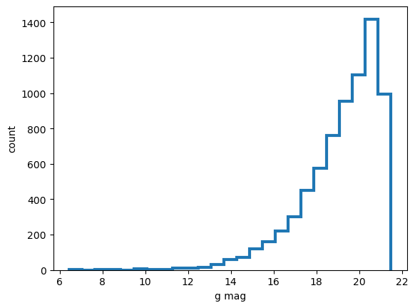
Plot the histogram of refcat sources:
[36]:
# calculate magnitudes
flux = df['phot_g_mean_flux'].values
mag = (flux*u.nJy).to(u.ABmag)
df['phot_g_mean_mag'] = mag.value

# plot the histogram
plt.xlabel('g mag')
plt.ylabel('count')
plt.hist(mag, histtype='step',lw=3, bins=25)
[36]:
(array([1.000e+00, 0.000e+00, 1.000e+00, 1.000e+00, 0.000e+00, 5.000e+00,
        4.000e+00, 3.000e+00, 9.000e+00, 9.000e+00, 1.600e+01, 3.300e+01,
        6.000e+01, 7.000e+01, 1.180e+02, 1.610e+02, 2.220e+02, 3.030e+02,
        4.520e+02, 5.770e+02, 7.600e+02, 9.540e+02, 1.105e+03, 1.419e+03,
        9.950e+02]),
 array([ 6.45667698,  7.05798584,  7.6592947 ,  8.26060355,  8.86191241,
         9.46322127, 10.06453012, 10.66583898, 11.26714784, 11.86845669,
        12.46976555, 13.07107441, 13.67238326, 14.27369212, 14.87500098,
        15.47630983, 16.07761869, 16.67892755, 17.2802364 , 17.88154526,
        18.48285412, 19.08416297, 19.68547183, 20.28678069, 20.88808955,
        21.4893984 ]),
 [<matplotlib.patches.Polygon at 0x7f632f551190>])
Plot both the reference catalog sources and the simulated centroid sources, normalizing the distribution to show the magnitude extent:
[37]:
plt.hist(mag, density=True, stacked=True, histtype='step',lw=2, bins=25, label='refcat')
plt.hist(mag[df['simulated'] ==True], density=True, stacked=True,lw=2, bins=25,histtype='step', label='simulated')
plt.legend()
plt.xlabel('g mag')
plt.ylabel('probability density')
[37]:
Text(0, 0.5, 'probability density')
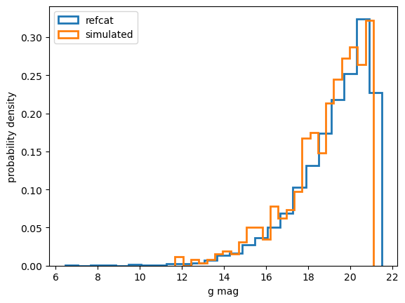
Notice that the simulated subset of the queried refcat region has a bright-end cutoff:
[38]:
print(min(mag))
print(min(mag[df['simulated'] ==True]))
6.456676983180913 mag(AB)
11.677913757880114 mag(AB)
Indeed, the refcat in this sky area contains sources all the way up to 6th magnitude. But with max_flux set to eg. 1e9 we only simulated sources up to about 11th magnitude (1e10 would result in approximately 10th magnitude). There are also some sources that do not contain the full GAIA filter information (either rp_flux or bp_flux is missing), and these also do not get simulated.
We can overplot the refcat sources on top of the postISR images:
[39]:
instrument= 'LSSTComCam'
detector=0
# 68661: 940
# 68659: 950
exposure_number = 5025082000942

# construct a dataId  for postISR extra-focal
data_id_extra = {
    "detector": detector,
    "instrument": instrument,
    "exposure": exposure_number,
    "visit":exposure_number
}

# read the postISR exposure
path_cwd = '/sdf/data/rubin/shared/scichris/DM-41679_lsstComCam/'
butlerRootPath = os.path.join(path_cwd, 'gen3repo')
butler = dafButler.Butler(butlerRootPath)
exposure_extra = butler.get("postISRCCD", data_id_extra, collections=['runIsr'])

donut_catalog = butler.get(
    "donutCatalog",  dataId=data_id_extra, collections=['runWEP_940-942_wcs']
    )
mean_ra_rad = np.mean(donut_catalog.coord_ra.values)
mean_dec_rad = np.mean(donut_catalog.coord_dec.values)

mean_ra_deg = np.rad2deg(mean_ra_rad)
mean_dec_deg = np.rad2deg(mean_dec_rad)
print(mean_ra_deg, mean_dec_deg)
295.29797781477106 -81.60506442557026
Given the exposure-attached WCS information we can calculate the x,y pixel coordinates from their ra, dec:
[40]:
wcs = exposure_extra.getWcs()
x,y = wcs.skyToPixelArray(df['coord_ra'], df['coord_dec'])

df['x_px'] = x
df['y_px'] = y
Plot all refcat sources from the query :
[41]:
fig,ax = plt.subplots(1,1, figsize=(6,6))
zscale = ZScaleInterval()
d = exposure_extra.image.array
vmin,vmax = zscale.get_limits(d)
plt.imshow(d,origin='lower', vmin=vmin, vmax=vmax)
plt.scatter(x,y,s=0.1,c='red')
plt.title(exposure_extra.getDetector().getName())
plt.xlabel('x [px]')
plt.ylabel('y [px]')
[41]:
Text(0, 0.5, 'y [px]')
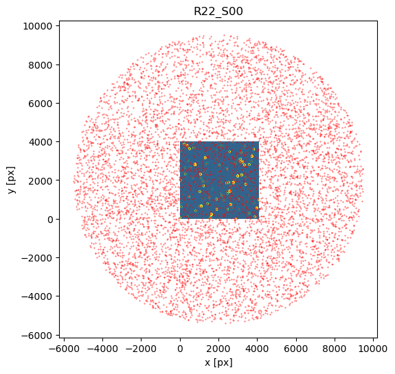
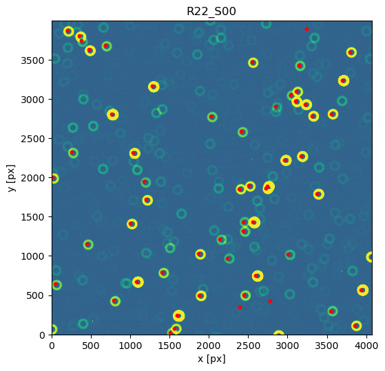
Notice that 1500 arcsec is sufficient to encompass all 9 comCam rafts (although to do that with a single refcat query we would have to query with ra/dec of the center of the raft - R22_S11). If we set the image limits to the CCD dimensions, and select only refcat sources brighter than 16th mag we notice that the simulated sources indeed correspond to the refcat sources.
[42]:
fig,ax = plt.subplots(1,1, figsize=(6,6))
ax.imshow(d,origin='lower', vmin=vmin, vmax=vmax)
mask1 = mag.value<16
mask2 = (0<x)*(x<4000)*(0<y)*(y<4000) # pick only sources in the CCD
m = mask1 * mask2
ax.scatter(x[m],y[m],s=10, c='red')
ax.set_title(exposure_extra.getDetector().getName())
ax.set_xlabel('x [px]')
ax.set_ylabel('y [px]')
[42]:
Text(0, 0.5, 'y [px]')
The steps above are packaged in these convenience functions, used when plotting refcat sources together with donut postage stamps:
[43]:
def get_exposure(
    instrument="LSSTComCam",
    detector=0,
    exposure_number=5025082000942,
    path_cwd="/sdf/data/rubin/shared/scichris/DM-41679_lsstComCam/",
    repo_name="gen3repo",
):
    """Read an exposure from butler.

    Parameters:
    -----------
    instrument: str
       Accepted instrument name (eg. "LSSTComCam",
       "LSSTCam").
    detector: int
       The detector id number.
    exposure_number: int
       The exposure number to load, consisting of observation
       date, and sequence number.
    path_cwd: str
       Absolute path to the output directory.
    repo_name: str
       Name of the sub-directory containing butler.yaml.

    Returns:
    --------
    lsst.afw.image._exposure.ExposureF

    """

    # construct a dataId  for postISR extra-focal
    data_id_extra = {
        "detector": detector,
        "instrument": instrument,
        "exposure": exposure_number,
        "visit": exposure_number,
    }
    # read the postISR exposure
    butler_root_path = os.path.join(path_cwd, repo_name)
    butler = dafButler.Butler(butler_root_path)
    exposure = butler.get("postISRCCD", data_id_extra, collections=["runIsr"])
    print(f"Read exposure {exposure_number}, detector {detector}, from {butler_root_path}")
    return exposure
[44]:
def get_refcat_df(exposure, query_radius_asec=1500,
                  path_cwd = "/sdf/group/rubin/shared/scichris/DM-41679_lsstComCam",
                  repo_name="gen3repo",
                  output_dir = "output-max-flux-1e9"):
    """Query refcat given the mean ra, dec from the
    centroid file corresponding to a particular exposure.

    Parameters:
    ---------
    exposure: lsst.afw.image._exposure.ExposureF
       Exposure for which we obtain the centroid sources and
       based on that query the refcat.
    query_radius_asec: float
       Refcat query radius in arcseconds.
    path_cwd: str
       Absolute path to the output directory.
    repo_name: str
       Name of the sub-directory containing butler.yaml.
    output_dir: str
       Name of the sub-directory containing the raw imSim output.

    Returns:
    --------
    df: pandas.core.frame.DataFrame
       The refcat-based dataFrame, including
       added columns such as g-magnitude ("phot_g_mean_mag")
       and WCS-based x,y px coordinates ("x_px", "y_px").

    """
    # obtain mean ra,dec from the centroid file
    meta = exposure.getInfo().getMetadata()
    visit = meta["RUNNUM"]
    zero_visit_str = str(visit).zfill(8)
    filter_letter = meta["FILTER"][0]
    chipid = meta["CHIPID"]

    zero_det_id = str(exposure.getDetector().getId()).zfill(3)
    fpath = os.path.join(
        path_cwd,
        output_dir,
        zero_visit_str,
        f"centroid_{zero_visit_str}-0-{filter_letter}-{chipid}-det{zero_det_id}.txt.gz",
    )
    print('\n Using centroid file {fpath}')
    centroid = Table.read(
        fpath,
        format="csv",
        delimiter=" ",
        names=[
            "object_id",
            "ra",
            "dec",
            "x",
            "y",
            "nominal_flux",
            "phot_flux",
            "fft_flux",
            "realized_flux",
        ],
    )
    print("\n Total number of objects in this CCD is ", len(centroid))

    mean_centroid_ra = np.mean(centroid["ra"])
    mean_centroid_dec = np.mean(centroid["dec"])

    # query the refcat
    mean_ra_deg = mean_centroid_ra
    mean_dec_deg = mean_centroid_dec
    collection = "refcats/gaia_dr2_20200414"
    dstype = "gaia_dr2_20200414"
    print(f'\n Querying the refcat collection {collection} \
    around ra:{mean_ra_deg}, dec:{mean_dec_deg} \
    with radius of {query_radius_asec} arcseconds')

    butler_root_path = os.path.join(path_cwd, repo_name)
    butler = dafButler.Butler(butler_root_path, collections=["refcats/gaia_dr2_20200414"])
    refs = set(butler.registry.queryDatasets(dstype))

    refCats = [dafButler.DeferredDatasetHandle(butler, _, {}) for _ in refs]

    dataIds = [butler.registry.expandDataId(_.dataId) for _ in refs]
    config = ReferenceObjectLoader.ConfigClass()
    config.filterMap = {f"{_}": f"phot_{_}_mean" for _ in ("g", "bp", "rp")}
    ref_obj_loader = ReferenceObjectLoader(
        dataIds=dataIds, refCats=refCats, config=config
    )

    ra = lsst.geom.Angle(mean_ra_deg, lsst.geom.degrees)
    dec = lsst.geom.Angle(mean_dec_deg, lsst.geom.degrees)

    center = lsst.geom.SpherePoint(ra, dec)

    radius = lsst.geom.Angle(query_radius_asec, lsst.geom.arcseconds)
    refcat_region = lsst.sphgeom.Circle(center.getVector(), radius)
    band = "bp"
    cat = ref_obj_loader.loadRegion(refcat_region, band).refCat
    df = cat.asAstropy().to_pandas().sort_values("id")

    # this creates a boolean mask to tell us which of the refcat sources got simulated
    centroid_ids = [int(object_id.split("_")[2]) for object_id in centroid["object_id"]]
    centroid["ids"] = centroid_ids
    df["simulated"] = np.in1d(df["id"], centroid["ids"])

    # calculate magnitudes
    flux = df["phot_g_mean_flux"].values
    mag = (flux * u.nJy).to(u.ABmag)
    df["phot_g_mean_mag"] = mag.value

    # calculate WCS-based pixel coords
    wcs = exposure_extra.getWcs()
    x, y = wcs.skyToPixelArray(df["coord_ra"], df["coord_dec"])

    df["x_px"] = x
    df["y_px"] = y

    return df
Starting from exposure, obtain the refcat with fluxes converted to AB magnitudes, and ra,dec source coordinates converted to WCS-based x,y pixel values:
[45]:
exposure = get_exposure()
df = get_refcat_df(exposure)
Read exposure 5025082000942, detector 0, from /sdf/data/rubin/shared/scichris/DM-41679_lsstComCam/gen3repo

 Using centroid file {fpath}

 Total number of objects in this CCD is  683

 Querying the refcat collection refcats/gaia_dr2_20200414     around ra:295.39614332357246, dec:-81.59774462532943     with radius of 1500 arcseconds
INFO:lsst.meas.algorithms.loadReferenceObjects.ReferenceObjectLoader:Loading reference objects from None in region bounded by [292.54347830, 298.24880834], [-82.01441301, -81.18107624] RA Dec
INFO:lsst.meas.algorithms.loadReferenceObjects.ReferenceObjectLoader:Loaded 7278 reference objects
[46]:
df[:5]
[46]:
| id | coord_ra | coord_dec | phot_g_mean_flux | g_camFlux | phot_bp_mean_flux | bp_camFlux | phot_rp_mean_flux | rp_camFlux | phot_g_mean_fluxErr | g_camFluxErr | phot_bp_mean_fluxErr | bp_camFluxErr | phot_rp_mean_fluxErr | rp_camFluxErr | coord_raErr | coord_decErr | epoch | pm_ra | pm_dec | pm_raErr | pm_decErr | pm_flag | parallax | parallaxErr | parallax_flag | astrometric_excess_noise | phot_variable_flag | simulated | phot_g_mean_mag | x_px | y_px | |
|---|---|---|---|---|---|---|---|---|---|---|---|---|---|---|---|---|---|---|---|---|---|---|---|---|---|---|---|---|---|---|---|---|
| 2227 | 6347682559333342336 | 5.141738 | -1.431137 | 60349.333720 | 60349.333720 | 48042.776329 | 48042.776329 | 91550.212451 | 91550.212451 | 183.098984 | 183.098984 | 2187.133629 | 2187.133629 | 2374.512800 | 2374.512800 | 1.287502e-09 | 1.468586e-09 | 57205.874409 | 1.076734e-09 | -3.436459e-08 | 2.591071e-09 | 2.905852e-09 | False | 1.230859e-09 | 1.568164e-09 | False | 0.00000 | NOT_AVAILABLE | False | 19.448319 | 4171.909220 | -5126.378421 |
| 2002 | 6347682559333401472 | 5.142896 | -1.431161 | 51250.534104 | 51250.534104 | 32040.119818 | 32040.119818 | 104398.748146 | 104398.748146 | 177.869842 | 177.869842 | 2092.624943 | 2092.624943 | 2335.022543 | 2335.022543 | 1.465456e-09 | 1.686865e-09 | 57205.874409 | 2.479213e-08 | -7.536406e-08 | 3.005054e-09 | 3.323866e-09 | False | 6.124334e-10 | 1.740461e-09 | False | 0.00000 | NOT_AVAILABLE | False | 19.625754 | 4005.856638 | -5153.258202 |
| 2091 | 6347682563630378240 | 5.142940 | -1.431073 | 120788.564772 | 120788.564772 | 62069.016586 | 62069.016586 | 222106.934921 | 222106.934921 | 235.845794 | 235.845794 | 2068.664712 | 2068.664712 | 2481.203986 | 2481.203986 | 8.612467e-10 | 9.634437e-10 | 57205.874409 | -3.792447e-09 | 4.519851e-08 | 1.790965e-09 | 1.841551e-09 | False | 2.784224e-09 | 1.039702e-09 | False | 0.47975 | NOT_AVAILABLE | False | 18.694935 | 3998.534421 | -5062.195875 |
| 2092 | 6347682563630378368 | 5.142853 | -1.431118 | 490539.308596 | 490539.308596 | 251022.902296 | 251022.902296 | 887274.733654 | 887274.733654 | 344.012632 | 344.012632 | 2648.685341 | 2648.685341 | 4366.685086 | 4366.685086 | 2.990641e-10 | 3.473743e-10 | 57205.874409 | 2.056232e-08 | 4.182208e-08 | 6.042890e-10 | 6.245315e-10 | False | 5.148430e-09 | 3.821001e-10 | False | 0.08107 | NOT_AVAILABLE | False | 17.173315 | 4011.538335 | -5109.179237 |
| 2296 | 6347682628052819712 | 5.141564 | -1.431030 | 23489.302076 | 23489.302076 | 20422.085320 | 20422.085320 | 37808.433087 | 37808.433087 | 170.154025 | 170.154025 | 2139.317278 | 2139.317278 | 2753.944297 | 2753.944297 | 3.321716e-09 | 4.127265e-09 | 57205.874409 | 9.275719e-09 | -3.188757e-08 | 6.905695e-09 | 9.419332e-09 | False | -2.380241e-09 | 3.665046e-09 | False | 0.00000 | NOT_AVAILABLE | False | 20.472825 | 4195.788395 | -5016.178139 |
Reading the data from butler#
We read the post-ISR image, estimated Zernikes, and donut stamps for a particular exposure (5025082000942) and detector R22_S00, for both the WCS-based generateDonutCatalogWcsTask and the direct detection generateDonutDirectDetectTask, distinguished below with different collection names.
[47]:
instrument = "LSSTComCam"
detector = 0
exposure_number = 5025082000942

# construct a dataId  for postISR extra-focal
data_id_extra = {
    "detector": detector,
    "instrument": instrument,
    "exposure": exposure_number,
    "visit": exposure_number,
}

# read the postISR exposure
path_cwd = "/sdf/data/rubin/shared/scichris/DM-41679_lsstComCam/"
butlerRootPath = os.path.join(path_cwd, "gen3repo")
butler = dafButler.Butler(butlerRootPath)
exposure_extra = butler.get("postISRCCD", data_id_extra, collections=["runIsr"])

# read the WCS-based results
collection = "runWEP_940-942_wcs"
donuts_extra = butler.get(
    "donutStampsExtra", dataId=data_id_extra, collections=[collection]
)
zernikes_raw = butler.get(
    "zernikeEstimateRaw", dataId=data_id_extra, collections=[collection]
)  # extra dets
zernikes_avg = butler.get(
    "zernikeEstimateAvg", dataId=data_id_extra, collections=[collection]
)  # extra dets

# read the direct detection results
collection = "runWEP_940-942_direct"
donuts_extra1 = butler.get(
    "donutStampsExtra", dataId=data_id_extra, collections=[collection]
)
zernikes_raw1 = butler.get(
    "zernikeEstimateRaw", dataId=data_id_extra, collections=[collection]
)  # extra dets
zernikes_avg1 = butler.get(
    "zernikeEstimateAvg", dataId=data_id_extra, collections=[collection]
)  # extra dets
Reading the OPD data#
We also include the “truth” files - the optical path difference (OPD). In this case we are reading the OPD from the header, but it could also be obtained via map_opd_to_zk function from ts_imsim, reproduced below. We show that the two provide equivalent result:
[48]:
def _map_opd_to_zk(
    opd_file_path, rot_opd_in_deg: float, num_opd: int, shift=0
) -> np.ndarray:
    """Map the OPD to the basis of annular Zernike polynomial (Zk).

    OPD: optical path difference.

    Parameters
    ----------
    rot_opd_in_deg : float
        Rotate OPD in degree in the counter-clockwise direction.
    num_opd : int
        Number of OPD positions calculated.

    Returns
    -------
    numpy.ndarray
        Zk data from OPD. This is a 2D array. The row is the OPD index and
        the column is z4 to z22 in um. The order of OPD index is based on
        the file name.
    """

    # Map the OPD to the Zk basis and do the collection
    # Get the number of OPD locations by looking at length of fieldX
    num_of_zk = 19
    opd_metr = OpdMetrology()
    opd_data = np.zeros((num_opd, num_of_zk))
    for idx in range(shift, num_opd + shift):
        # print(idx)
        opd = fits.getdata(opd_file_path, idx)

        # Rotate OPD if needed
        if rot_opd_in_deg != 0:
            opd_rot = opd.copy()
            # Since to rotate the opd we need to substitue the nan values
            # for zeros, we need to find the minimum value of the opd
            # excluding the nan values. Then after the rotation we will
            # discard the values that are smaller than the minimum value.
            # Note that we use order = 0 to avoid interpolation errors.
            min_value = np.nanmin(np.abs(opd_rot))
            opd_rot[np.isnan(opd_rot)] = 0.0
            opd_rot = rotate(opd_rot, rot_opd_in_deg, reshape=False, order=0)
            opd_rot[np.abs(opd_rot) <= min_value] = np.nan
        else:
            opd_rot = opd

        # z1 to z22 (22 terms)
        zk = opd_metr.get_zk_from_opd(opd_map=opd_rot)[0]

        # Only need to collect z4 to z22
        init_idx = 3
        opd_data[idx - shift, :] = zk[init_idx : init_idx + num_of_zk]

    return opd_data
[49]:
# find the rotation angle from the exposure
meta = exposure_extra.getInfo().getMetadata()
rotation = meta['ROTANGLE']

opd_file_path = '/sdf/data/rubin/shared/scichris/DM-41679_lsstComCam/output-max-flux-1e9/00068661/opd_0.0.fits.fz'
opds1 = _map_opd_to_zk(opd_file_path, rotation, 9, 1)
[50]:
# read the opd file from the in-focus opd
hdul = fits.open(opd_file_path)
opds = {}
for i in range(len(hdul)):
    opd_zks_1_28 = []
    for key,value in hdul[i].header.items():

        if key.startswith('AZ'):
            #print(key.split('_')[1])
            opd_zks_1_28.append(value)
    opds[i] = opd_zks_1_28
Plot the OPDs comparison for a single ComCam raft:
[51]:
i=0
plt.figure()
plt.plot(np.arange(4,23), np.array(opds[i+1][3:22]), '-d', label='header-based')
plt.plot(np.arange(4,23), opds1[i], '--', label='map-based')
plt.legend()
plt.title(f'OPD, detector {detector}')
plt.ylabel('zk value [nm]')
plt.xlabel('zk polynomial')
plt.xticks(np.arange(4,23,2))
[51]:
([<matplotlib.axis.XTick at 0x7f631c656a90>,
  <matplotlib.axis.XTick at 0x7f631cac4d50>,
  <matplotlib.axis.XTick at 0x7f631e904ed0>,
  <matplotlib.axis.XTick at 0x7f631cad9bd0>,
  <matplotlib.axis.XTick at 0x7f631cadbf90>,
  <matplotlib.axis.XTick at 0x7f631caa1f90>,
  <matplotlib.axis.XTick at 0x7f631caa2450>,
  <matplotlib.axis.XTick at 0x7f631caa5990>,
  <matplotlib.axis.XTick at 0x7f631caa7cd0>,
  <matplotlib.axis.XTick at 0x7f631cab2cd0>],
 [Text(4, 0, '4'),
  Text(6, 0, '6'),
  Text(8, 0, '8'),
  Text(10, 0, '10'),
  Text(12, 0, '12'),
  Text(14, 0, '14'),
  Text(16, 0, '16'),
  Text(18, 0, '18'),
  Text(20, 0, '20'),
  Text(22, 0, '22')])
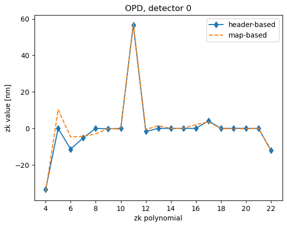
The slight difference identified at the time of writing is due to imsim fitting by default Z4 through Z28, whereas ts_imsim fitting Z4 through Z22. This is fixed by DM-42848 (that extends the default fitting range for ts_imsim).
[52]:
def plot_raw_zernikes(
    output_zernikes_raw,
    ax=None,
    fig=None,
    title="",
    output_zernikes_averaged=None,
    bbox_to_anchor=[0.55, 0.65],
    legendfontsize=12,
    opd=None,
):
    """Plot the raw Zernike coefficients.

    Parameters
    ----------
    output_zernikes_raw: numpy.ndarray
       Zernike fit coefficients for the donuts.
    ax: axis for plotting, if None it is added to the figure
    fig: figure for plotting
    """
    if fig is None:
        fig = plt.figure()

    if ax is None:
        ax = fig.add_axes([0, 0, 0.6, 1])

    for i in range(len(output_zernikes_raw)):

        ax.plot(
            np.arange(4, 23),
            1000 * output_zernikes_raw[i],
            "--s",
            alpha=0.4,
            label=f"donut {i}",
        )
    if output_zernikes_averaged is not None:
        ax.plot(
            np.arange(4, 23), 1000 * output_zernikes_averaged, "-d", label="average"
        )
    if opd is not None:
        ax.plot(np.arange(4, 23), opd, "-o", label="opd", c="red", alpha=1)
    ax.set_xlabel(
        "Zernike polynomials mode",
    )
    ax.set_ylabel(
        "Zernike Coefficient [nanometers]",
    )
    ax.legend(
        fontsize=legendfontsize,
        loc="center left",
        bbox_to_anchor=bbox_to_anchor,
        ncol=2,
    )
    ax.set_xticks(np.arange(4, 23)[::2])
    ax.grid()

    ax.set_title(title, fontsize=18)

    return


def plot_donut_locations(
    exposure,
    donut_stamps,
    ax=None,
    fig=None,
    left=0.6,
    bottom=0.5,
    height=0.6,
    noxticks=True,
    noxlabel=True,
    notitle=True,
):
    """Plot the donut locations on the postISR image.

    Parameters
    ----------
    exposure: lsst.afw.image.Exposure
        Exposure (postISR) with the donut images.
    donut_stamps: Collection of postage stamps as
        lsst.afw.image.maskedImage.MaskedImage.
        with additional metadata.
    ax: axis for plotting, if None it is added to the figure.
    fig: figure for plotting , if None a new figure is made.
    """
    if fig is None:
        fig = plt.figure()

    if ax is None:
        ax = fig.add_axes([left, bottom, 0.4, height])  # left, bottom, width,  height

    data = exposure.image.array
    zscale = ZScaleInterval()
    vmin, vmax = zscale.get_limits(data)

    ax.imshow(data, origin="lower", vmin=vmin, vmax=vmax)

    nrows = len(donut_stamps)
    for i in range(nrows):
        donut = donut_stamps[i]
        xy = donut.centroid_position

        # plot the cross marking that the donut was used
        ax.scatter(xy[0], xy[1], s=200, marker="+", c="m", lw=4)

        # plot the donut number on the plot
        xtext, ytext = xy[0], xy[1]
        ytext -= 60
        if xtext + 100 > 4096:
            xtext -= 250
        if len(str(i)) > 1:  # move to the left label that is too long
            xtext -= 340
        else:
            xtext -= 260
        ax.text(xtext, ytext, f"{i}", fontsize=17, c="white")
    ax.yaxis.tick_right()
    if not noxlabel:
        ax.set_xlabel("x [px]")
    ax.set_ylabel("y [px]")
    if noxticks:
        ax.set_xticklabels("")
    ax.yaxis.set_label_position("right")
    info = exposure.getMetadata()
    if not notitle:
        ax.set_title(f"exposure {info['DAYOBS']}{info['SEQNUM']}")
    return


def plot_donut_stamps(donut_stamps, text=""):
    """Plot the donut stamp image cutouts.

    Parameters
    ----------
    donut_stamps: Collection of postage stamps as
        lsst.afw.image.maskedImage.MaskedImage.
        with additional metadata.
    """
    # calculate number of rows given
    # the constraint of the number of
    # columns
    n_donuts = len(donut_stamps)
    ncols = 6
    nrows = n_donuts // ncols
    if nrows * ncols < n_donuts:
        nrows += 1

    fig, axs = plt.subplots(nrows, ncols, figsize=(3 * ncols, 3 * nrows))
    ax = np.ravel(axs)
    for i in range(n_donuts):
        donut = donut_stamps[i]
        ax[i].imshow(donut.stamp_im.image.array, origin="lower")
        ax[i].text(80, 80, f"{i}", fontsize=17, c="white")
    fig.subplots_adjust(hspace=0.35)

    # if there are more axes than donuts,
    # turn off the extra axes
    ncells = nrows * ncols
    if ncells > n_donuts:
        for axis in ax[n_donuts:]:
            axis.axis("off")
    ax[0].set_title(text)
    return
Fit results: WCS-based#
Below we illustrate the fit results using the WCS-based source selection.
[53]:
%matplotlib inline

fig = plt.figure(figsize=(14, 5))

t = f"{exposure_extra.visitInfo.instrumentLabel} {exposure_extra.detector.getName()}, WCS-based refcat sources"
plot_raw_zernikes(
    zernikes_raw,
    fig=fig,
    title=t,
    output_zernikes_averaged=zernikes_avg,
    opd=opds[1][3:22],
)
plot_donut_locations(
    exposure_extra,
    donuts_extra,
    fig=fig,
    left=0.6,
    bottom=0.0,
    height=1,
    notitle=False,
    noxlabel=False,
    noxticks=False,
)
plot_donut_stamps(donuts_extra)

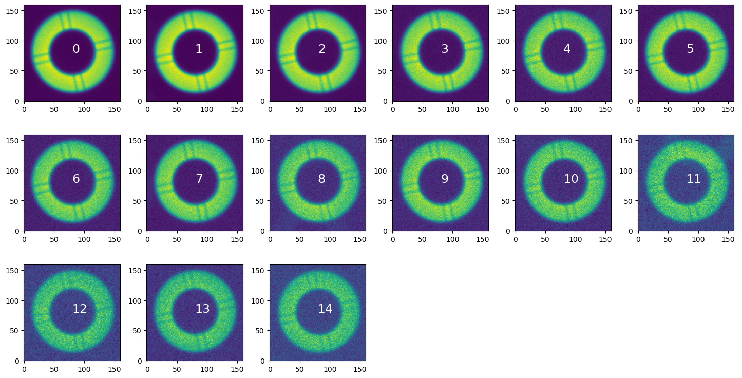
Fit results: direct detection#
Here we illustrate fit results using direct detection. Donut blends contribute to wavefront estimation most offset from the opd. Removing these provides a much smaller scatter.
[54]:
%matplotlib inline

fig = plt.figure(figsize=(14, 5))

t = f'{exposure_extra.visitInfo.instrumentLabel} {exposure_extra.detector.getName()} direct detection'
plot_raw_zernikes(zernikes_raw1, fig=fig, title=t, output_zernikes_averaged=zernikes_avg1, opd=opds[1][3:22])
plot_donut_locations(exposure_extra, donuts_extra1, fig=fig, left=0.6, bottom=0., height=1, notitle=False, noxlabel=False, noxticks=False)
plot_donut_stamps(donuts_extra1)
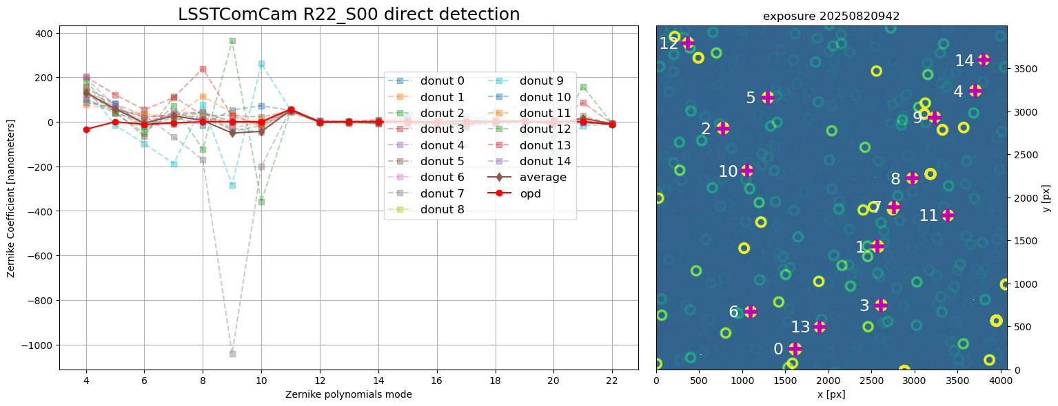
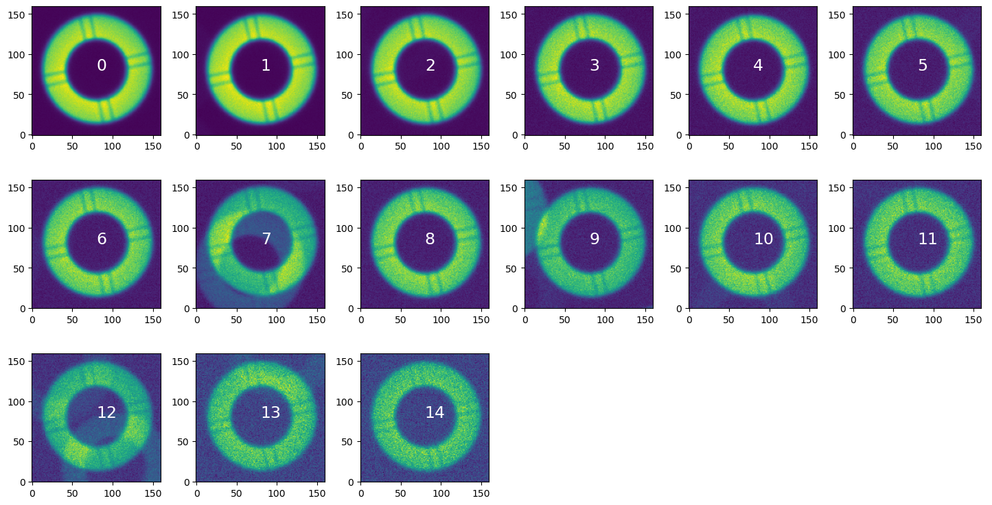
Note that here direct source detection provided some blended images, i.e. donuts contaminated by faint background sources.
Blended donuts#
Here we show the magnitudes of simulated refcat sources around blends. One parameter of donut source selector, isolatedMagDiff, sets the minimum magnitude difference for overlapping sources to be considered as isolated. Another parameter, unblendedSeparation, sets the minimum distance between centers of two donuts to be considered as isolated.
[55]:
def plot_image_zoomed(
    exposure,
    df,
    w=500,
    xcen=1000,
    ycen=1000,
    maglim=16,
    ax2title="zoomed region",
    label_refcat_mags=False,
    xshift=100,
    dmag=3,
    bright_refcat_color="red",
    faint_refcat_color="lightskyblue",
    refcat_text_params={"color": "black", "fontsize": 14},
):
    """Plot postISR image and the zoomed-in region

    Parameters
    ------------
      exposure : lsst.afw.image._exposure.ExposureF
            The exposure to plot.
      df : pandas.core.frame.DataFrame
            Refcat used to plot sources. Note, it needs
            to have the phot_g_mean_mag  column for magnitudes,
            and x_px, y_px for WCS-based coordinates of refcat
            sources for that particular exposure, as calculated
            above.
      w : int
            Half-width of the zoomed-in region size.
      xcen: int
            X-coordinate of center of the zoomed-in region.
      ycen: int
            Y-coordinate of center of the zoomed-in region.
      maglim: float
            Upper magnitude limit for refcat sources
            (to avoid plotting very faint sources that
            were not simulated).
      ax2title: str
            Title for the right-hand side panel.
      label_refcat_mags: bool
            Whether to label the refcat sources with
            their `phot_g_mag` magnitude.
      xshift: int
            The amount of shift in pixels to the left of
            the donut magnitude label.
      dmag: float
            The number of magnitudes for fainter sources
            to be labeled in the zoomed-in panel.
      bright_refcat_color: str
            The color to use for labeling bright refcat sources.
      faint_refcat_color: str
            The color to use for labeling bright refcat sources.
      refcat_text_params: dict
            A dictionary of kwargs to pass when plotting refcat sources.

    """
    d = exposure.image.array
    zscale = ZScaleInterval()
    vmin, vmax = zscale.get_limits(d)

    # anchor coordinates : (xleft, ybottom)
    xleft = xcen - w
    xright = xcen + w

    ybot = ycen - w
    ytop = ycen + w

    # zooomed-in subset of the entire image
    dzoomed = d[ycen - w : ycen + w, xcen - w : xcen + w]

    # select elements of refcat that are within
    # upper magnitude bounds,
    # and within the CCD dimensions
    mag = df["phot_g_mean_mag"].values
    mask_mag = mag < maglim

    # pick only sources in the CCD
    ccd_x, ccd_y = np.shape(d)
    mask_ccd = (
        (0 < df["x_px"].values)
        * (df["x_px"].values < ccd_x)
        * (0 < df["y_px"].values)
        * (df["y_px"].values < ccd_y)
    )
    m = mask_mag * mask_ccd

    # left: plot full image  with the zoomed region marked by a rectangle
    fig, ax = plt.subplots(1, 2, figsize=(12, 6))

    ax[0].imshow(d, origin="lower", vmin=vmin, vmax=vmax)

    # Create a Rectangle patch
    #:                +------------------+
    #:                |                  |
    #:              height               |
    #:                |                  |
    #:               (xy)---- width -----+
    # patches.Rectangle(xy, width, height)
    rect = patches.Rectangle(
        (xleft, ybot), 2 * w, 2 * w, linewidth=1, edgecolor="r", facecolor="none"
    )

    # Add the patch to the Axes
    ax[0].add_patch(rect)

    ax[0].scatter(df["x_px"].values[m], df["y_px"].values[m], s=10, c="red")

    ax[0].set_title(exposure_extra.getDetector().getName())
    ax[0].set_xlabel("x [px]")
    ax[0].set_ylabel("y [px]")
    xsize, ysize = np.shape(dzoomed)

    # right: plot zoomed-in section together with refcat sources
    # appropriately shifted given the origin shift
    # ax[1].scatter(x[m]-xleft,y[m]-ybot,s=100, c='red')
    # extent=  (left, right, bottom, top)
    ax[1].imshow(
        dzoomed,
        extent=(xleft, xcen + w, ybot, ycen + w),
        origin="lower",
        vmin=vmin,
        vmax=vmax,
    )

    # pick sources in the zoomed-in region
    mask_zoom = (
        (xleft < df["x_px"].values)
        * (df["x_px"].values < xright)
        * (ybot < df["y_px"].values)
        * (df["y_px"].values < ytop)
    )
    m = mask_mag * mask_zoom

    # also plot sources fainter by three mags in the zoomed-in region
    mask_mag_faint = (maglim < mag) * (mag < maglim + dmag)
    m2 = mask_mag_faint * mask_zoom
    # with the "extent" appropriately set,
    # we don't need to shift the refcat source coordinates

    # plot bright and faint refcat sources with different colors
    ax[1].scatter(x[m], y[m], s=100, c=bright_refcat_color, label=f"refcat < {maglim}")
    ax[1].scatter(
        x[m2],
        y[m2],
        s=100,
        c=faint_refcat_color,
        label=f"{maglim} < refcat < {maglim+dmag}",
    )

    # add source magnitude as  a label
    if label_refcat_mags:
        for mask, refcat_color in zip(
            [m, m2], [bright_refcat_color, faint_refcat_color]
        ):
            if np.sum(mask) > 0:  # only label if there are any sources in each category
                for i in range(len(x[mask])):
                    xtext, ytext = x[mask][i] - xshift, y[mask][i] + 20
                    ax[1].text(
                        xtext,
                        ytext,
                        f"{mag[mask][i]:.2f}",
                        path_effects=[
                            pe.withStroke(linewidth=2, foreground=refcat_color)
                        ],
                        **refcat_text_params,
                    )
    ax[1].set_xticks
    ax[1].legend(fontsize=12)
    ax[1].set_title(ax2title)
    ax[1].set_xlabel("x [px]")
    ax[1].set_ylabel("y [px]")
Read in the postISR exposure for a single detector. Given the centroid source coordinates, query the GAIA DR2 reference catalog to obtain the coordinates and fluxes of catalog sources. Convert g-mag fluxes to AB magnitudes, and sky coordinates (ra,dec) to pixel coordinates (x,y).
[56]:
exposure = get_exposure()
df = get_refcat_df(exposure)
Read exposure 5025082000942, detector 0, from /sdf/data/rubin/shared/scichris/DM-41679_lsstComCam/gen3repo

 Using centroid file {fpath}

 Total number of objects in this CCD is  683

 Querying the refcat collection refcats/gaia_dr2_20200414     around ra:295.39614332357246, dec:-81.59774462532943     with radius of 1500 arcseconds
INFO:lsst.meas.algorithms.loadReferenceObjects.ReferenceObjectLoader:Loading reference objects from None in region bounded by [292.54347830, 298.24880834], [-82.01441301, -81.18107624] RA Dec
INFO:lsst.meas.algorithms.loadReferenceObjects.ReferenceObjectLoader:Loaded 7278 reference objects
We can illustrate a region of any size, eg. 1000 pixels wide. In the left-hand-side panel the red dots represent WCS-based pixel coordinates of the reference catalog sources up to the WEP donut source selector cutoff magnitude (16th), as well as 3 magnitudes deeper (16th-19th mag):
[57]:
plot_image_zoomed(exposure, df, w=500, xcen=1000, ycen=1000,
                  maglim = 16, label_refcat_mags=True,
                  xshift=65)
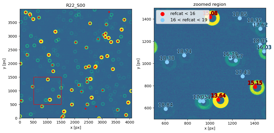
Zoom around each donut, plotting the magnitude of the nearby reference catalog sources. Since we select only reference catalog sources brighter than 16th magnitude, some sources are not labeled:
[58]:
for i in range(len(donuts_extra1)):
    stamp = donuts_extra1[i]
    xdon, ydon = stamp.centroid_position
    plot_image_zoomed(
        exposure_extra,
        df,
        w=200,
        xcen=int(xdon),
        ycen=int(ydon),
        maglim=16,
        ax2title=f"donut {i}",
        label_refcat_mags=True,
        xshift=20,
    )
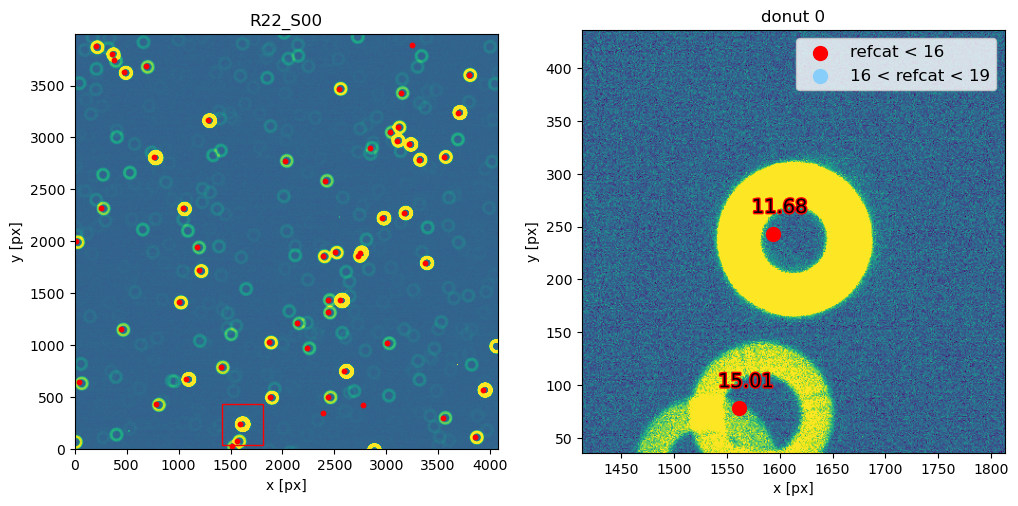
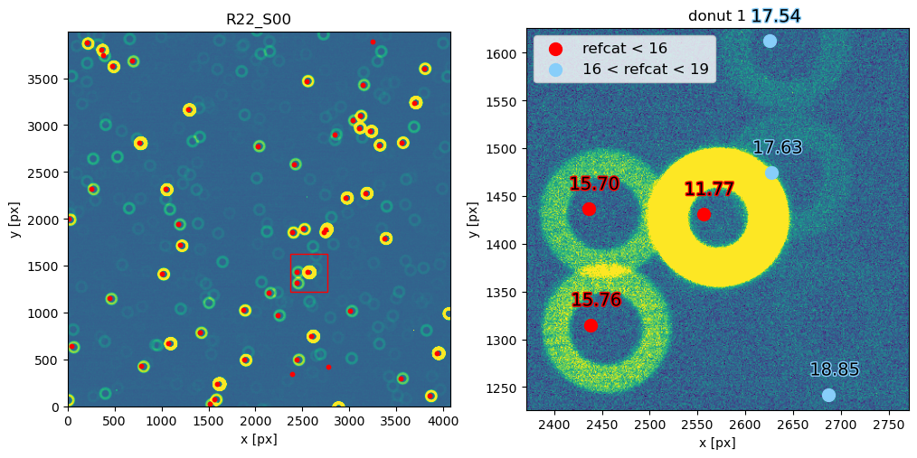

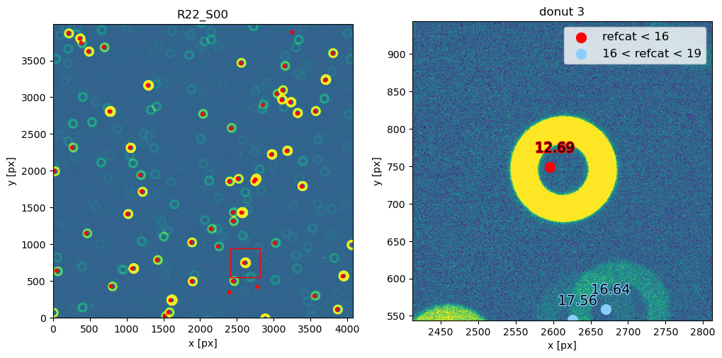
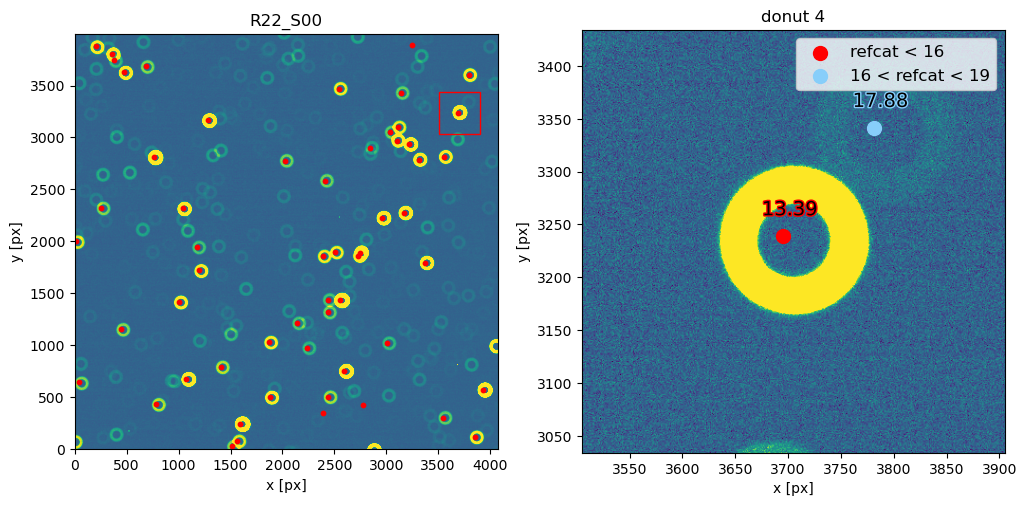
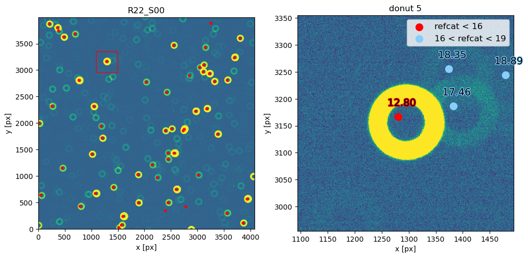
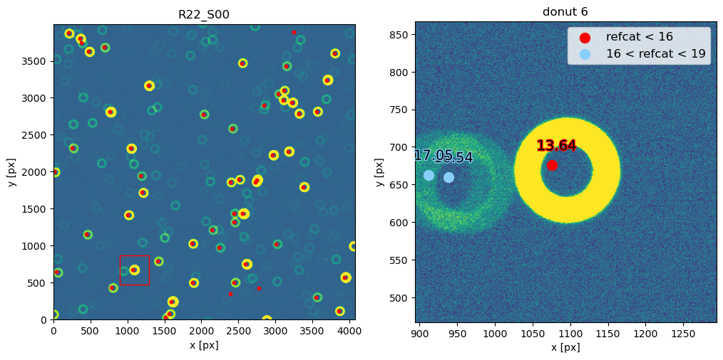
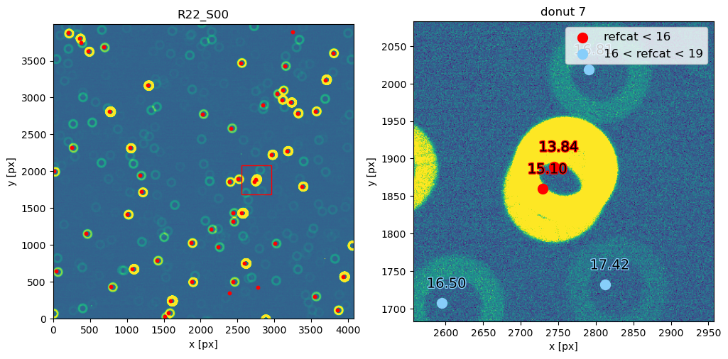
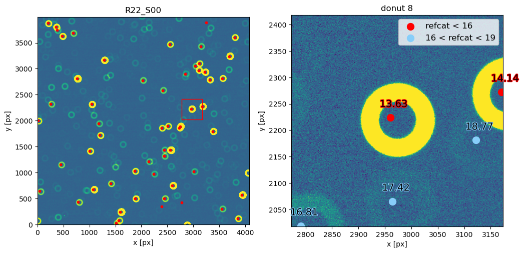
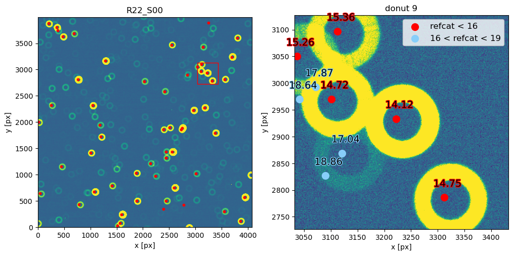
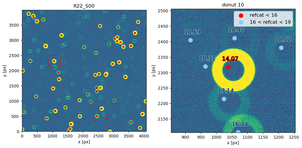
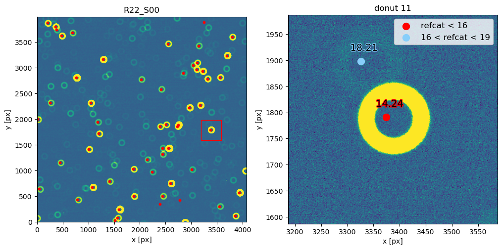
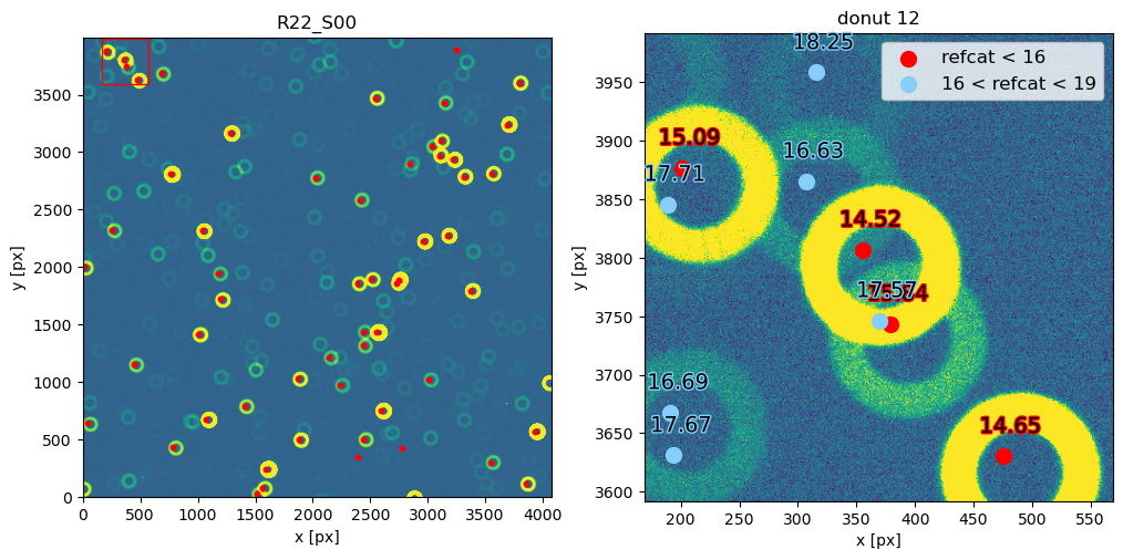
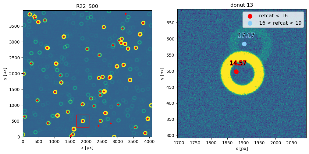
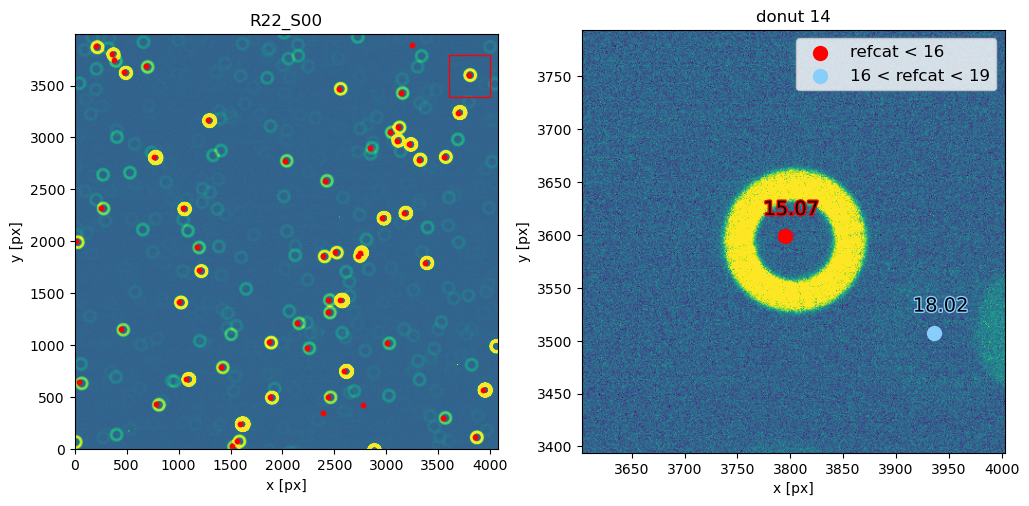
If we remove the blended donuts the overall estimate is similar to the WCS-based. Note, that such blended (or otherwise imperfect) donuts would be picked out by the Signal-to-Noise estimation implemented by DM-42228.
[59]:
fig = plt.figure(figsize=(14, 5))

t = f"{exposure_extra.visitInfo.instrumentLabel} {exposure_extra.detector.getName()} direct detection, no blends"
idx_choose = [0, 1, 2, 3, 4, 5, 6, 8, 10, 11, 13, 14]
plot_raw_zernikes(
    zernikes_raw1[idx_choose],
    fig=fig,
    title=t,
    output_zernikes_averaged=zernikes_avg1,
    opd=opds[1][3:22],
)
donuts_choose = [donuts_extra1[i] for i in idx_choose]
plot_donut_locations(
    exposure_extra,
    donuts_choose,
    fig=fig,
    left=0.6,
    bottom=0.0,
    height=1,
    notitle=False,
    noxlabel=False,
    noxticks=False,
)
plot_donut_stamps(donuts_choose)
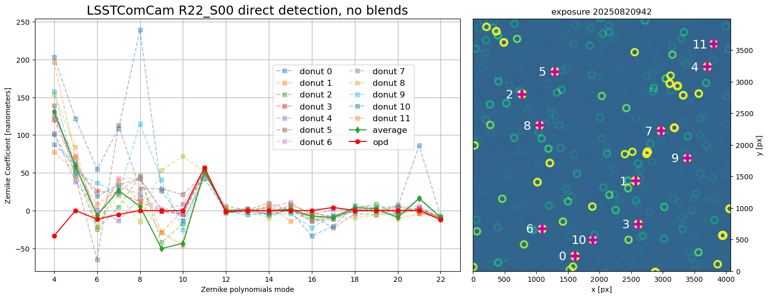
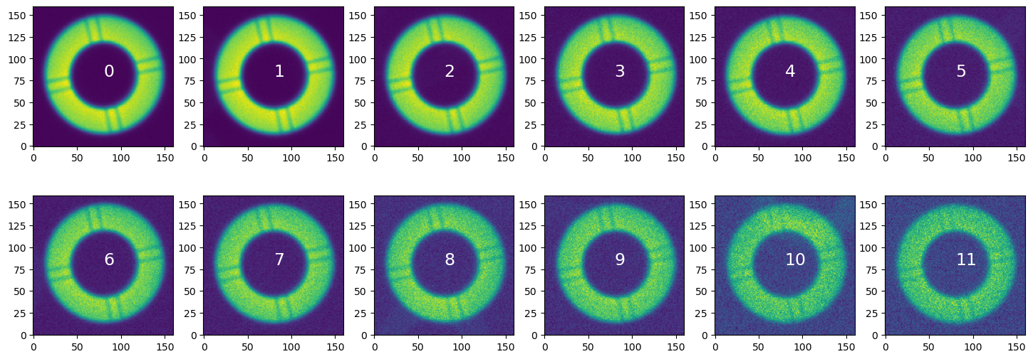
Summary#
To further the Active Optics System testing we developed the imSim simulations that use opsim database as a visit catalog (including pointing information, filter used, exposure time, cadence), querying at each location GAIA reference catalog for source location, magnitude distribution, and spectral information. We showed how multiple visits can be simulated for several instruments (LSSTCam, LSSTComCam), applying various defocal offsets. We performed the instrument signature removal using standard calibration procedures, and run wavefront estimation as a pipetask that can be executed either via slurm submission files, bps condor, or interactively. We illustrate the data products created by the pipeline, such as individual estimated Zernike modes, donut stamps, and opd files. We finally consider the issue of blended donuts, and other stamp-level imperfections (eg. bad amplifier or other image defects) that would be mitigated by the signal-to-noise estimation, sigma-clipping, and other stamp- or wavefront estimation-level methods.